Beam characterization

The nominal Full Width Half Maximum (FWHM) of a LOFAR Station beam is determined using the equation

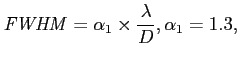where λ denotes wavelength and D denotes the station diameter. The value of α₁ will depend on the tapering intrinsic to the layout of the station, and any additional tapering which may be used to form the station beam. No electronic tapering is presently applied to LOFAR station beamforming. For a uniformly illuminated circular aperture, α₁ takes the value of 1.02, and the value increases with tapering (Napier 1999).

The Field of View (FoV) of a LOFAR station is defined by

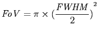The number of pointings to cover 2π steradians of sky in a Nyquist sampled way (on a square grid) is approximately 64800/FoV. After the weighted combination of the different pointings, the effective sensitivity will be better by a factor 1.5. Hence, one can choose to sample at slightly less than Nyquist to increase surveying speed.

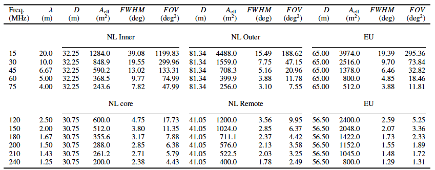
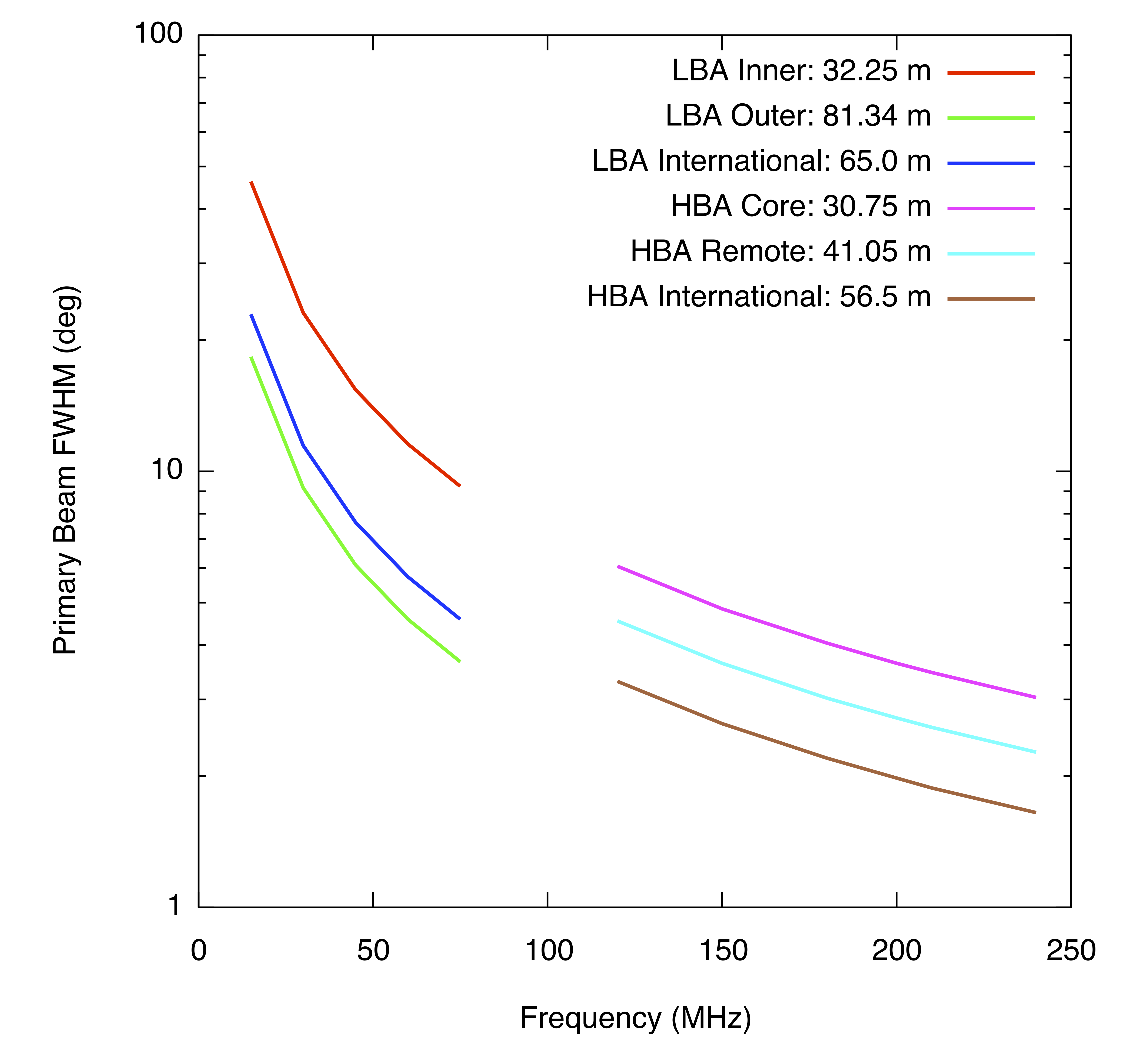
Table 1 and Figure 1 summarize the FWHM and the FoV, for the different layouts of LOFAR stations .

Array Angular Resolution

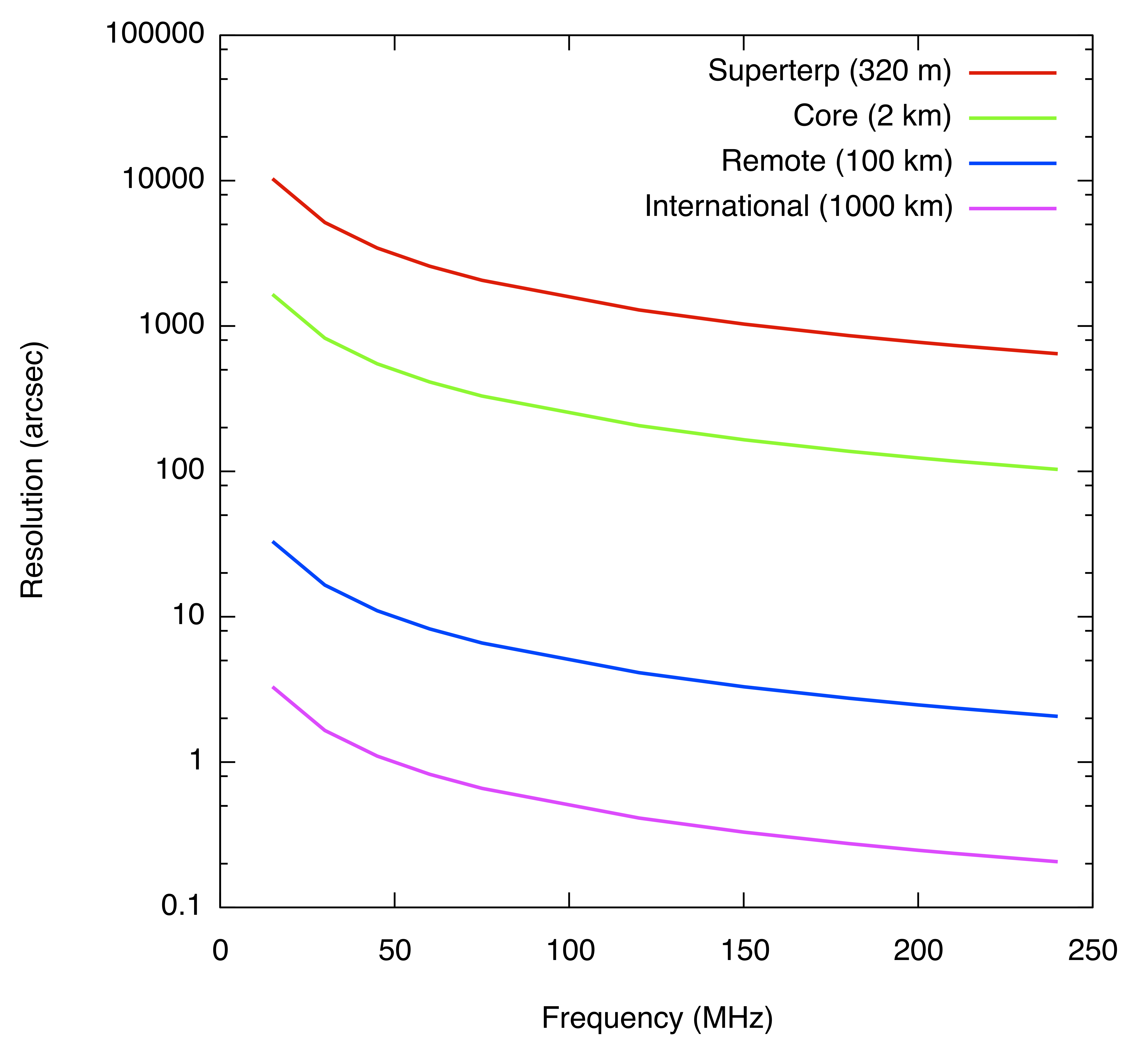
The angular resolution of the LOFAR array, calculated as the full width half maximum (FWHM) of the synthesized beam in radians, is given by

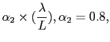
where λ is the observing wavelength, L denotes the longest baseline, and α₂ depends on the array configuration and the imaging weighting scheme (natural, uniform, robust, ...). Values of the resolution of LOFAR based on a value of α₂=0.8, which corresponds to uniform weighting scheme for the Dutch array can be found in Table 2.

Note: The numbers on the table below are indicative. For example in the NL the maximum baseline of ~82 km is only at a North-South direction. At the east-west direction the resolution is significantly lower; currently the maximum east-west baseline is ~21 km.

Caution: The numbers quoted here are projected for the full array and assume ideal performance of the instrument. The LOFAR Unified Calculator for Imaging (LUCI), which is based on these numbers, can be used to compute the thermal noise of your data. 

For more practical information on the actual sensitivity of the current configuration, readers should consult the corresponding "Interferometric Mode", "Beam Formed Mode" and "Direct Storage Mode"  pages.

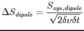
System Equivalent Flux Density

The System Equivalent Flux Density (SEFD or system sensitivity) is defined as

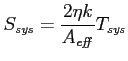
where k denotes Boltzmann's constant, η denotes the system efficiency factor (~ 1.0) , A_eff denotes the total collecting area, and T_sys denotes the system noise temperature. The latter consists of a sky brightness component and an instrumental component:

For all LOFAR frequencies the sky brightness temperature is dominated by the Galactic radiation, which depends strongly on the wavelength:

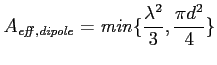
Table 3 provides a lower limit for the effective area of the different LBA array selections. The upper limit is given by the number of dipoles times λ²/ 3, and it is given in the last column (for 48 dipoles). Note that the inner array consists of only 46 dipoles. The effective area of each dipole in the array is determined by its distance to the nearest dipole (d) within the full array:

Table 3 Effective area (m²) for the different LBA array selections as function of frequency (MHz) or wavelength (m). (*) An 81.34 m station has an area of 5196.3 m².

For an HBA dipole, the effective area is limited by the available area in a tile. There are 16 dipole antennas within one 5 m by 5 m tile, hence, the dipole effective area is given by

The resulting HBA station effective area is given in Table 4:

Table 4 Effective area (m²) for the HBA array as function of frequency (MHz) or wavelength (m). At 120 MHz the effective area is limited by the tile size. (*) There are two HBA fields per core station.

Empirical SEFD values for the Dutch stations have been derived by utilizing a 2-minute imaging-mode observation of 3C295 in LBA and in HBA, taken near transit. The results are plotted in Figure 3. Some of the visibilities were flagged to remove RFI. The contributions of Cygnus A and Cassiopeia A were modelled and removed (in the case of the LBA). From these preprocessed data, the S/N ratio of the visibilities was determined for each baseline between similar stations (i.e., core-core and remote-remote baselines for the HBA). The S/N was defined as the mean of the parallel-hand (XX,YY) visibilities, divided by the standard deviation of the cross-hand (XY,YX) visibilities. These S/N values were then combined with the spectral model of 3C295 from Scaife & Heald (2012), and taking the bandwidth and integration time of the individual visibilities into account, an estimate of the SEFD for the type of station comprising this baseline selection was obtained. The most distant remote stations are excluded from this analysis as 3C295 is resolved on all baselines to those stations. For the same reason, we have not attempted to determine empirical SEFDs for international stations using this procedure.

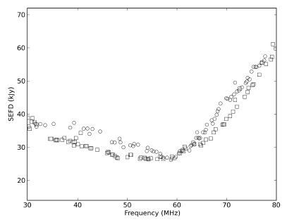
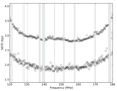
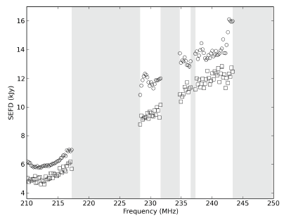
Figure 3: Plots of the SEFD as a function of frequency for the various LOFAR operating bands and station configurations. The grayed regions are excluded from plotting due to strong post-flagging RFI contamination. In the case of HBA, the circles are for core stations and squares are for remote stations. In the LBA, the circles are LBA INNER core stations and the squares are LBA OUTER core stations.

Sensitivities

Caution: The numbers quoted here are projected for the full array and assume ideal performance of the instrument

The LOFAR Unified Calculator for Imaging (LUCI), which is based on these numbers, can be used to compute the thermal noise of your data.

For more practical information on the actual sensitivity of the current configuration, readers should consult the "Examples of deliverable LOFAR products" page.

The sensitivity ΔS (in Jy) of a single dipole (or half an "antenna'') is defined as follows:

where δν denotes the bandwidth (in Hz) and δ t (in s) denotes the total integration time. An antenna that consists of two (equal) dipoles placed perpendicular to each other has a sensitivity of

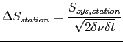
For one station, the overlap in effective area from different dipoles has to be taken into account. Using the SEFD of a station (see previous section) for a single polarization, we can calculate its sensitivity:

In the case of an image, the signals from different baselines and two polarizations are combined. For LOFAR this includes signals from stations with different effective areas. Therefore, the noise level in a LOFAR image is given by

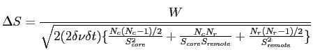
where W denotes a factor for increase of noise due to the weighting scheme (which depends on the type of weighting: natural, uniform, robust, ...), N_c and N_r denote the number of core and remote stations respectively, S_core and S_remote denote the SEFDs for the core and the remote stations respectively. This expression can easily be extended to include European stations.

In case of an array having N equal stations (or dishes) the following familiar result is retrieved

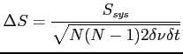
Table 5 provides the expected noise levels in LOFAR images. The quoted sensitivities are for image noise calculated assuming 8 hours of integration and an effective bandwidth of 3.66 MHz (20 subbands). The sensitivities are based on the zenith SEFD’s derived from 3C295 in the Galactic halo as presented in Fig. 3. These values assume a factor of 1.3 loss in sensitivity due to time-variable station projection losses for a declination of 30 degrees, as well as a factor 1.5 to take into account losses for “robust” weighting of the visibilities, as compared to natural weighting. Values for 15 MHz have not yet been determined awaiting a good station calibration. Similarly values at 200, 210, and 240 MHz should be viewed as preliminary and are expected to improve as the station calibration is improved.

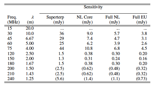
Table 5: LOFAR sensitivities. The different columns refer to the case of a 6-station Superterp, a 24-station core array, a 40-station Dutch array, and a 48-station full array. 

The values quoted for the HBA in Table 5 agree with empirical values derived from recent observations on 3C196 and the North Celestial Pole (NCP) where all NL remote stations were tapered to match 24-tile core stations. With improved station calibration, these estimates can likely be improved in the future by a factor of about 1.2. For the more compact LOFAR configurations, confusion noise will exceed the quoted values. The quoted sensitivities for the lower LBA frequencies have not yet been achieved in practice.

Bandpass

There are several contributions to the frequency dependent sensitivity of LOFAR to incoming radiation (the bandpass). At the correlator, a digital correction is applied within each 0.2 MHz subband to remove the frequency-dependent effects of the conversion to the frequency domain. The station beam is also strongly frequency dependent, except at the beam-pointing centre. Finally, the physical structure of the individual receiving elements causes a strongly peaked contribution to the bandpass near the resonance frequency of the dipole. In the case of the LBA dipoles, the nominal resonance frequency is at 52 MHz. However, as can already be seen in Figure 4, the actual peak of the dipole response is closer to 60 MHz.

Determining the combined bandpass (referred to as the “global bandpass”), which includes all frequency dependent effects in the system that are not yet corrected post-correlation, can be achieved during calibration. To illustrate this, the bright quasar 3C196 has been observed using the core and remote stations in the LBA and in the three HBA bands (see Figure 4).

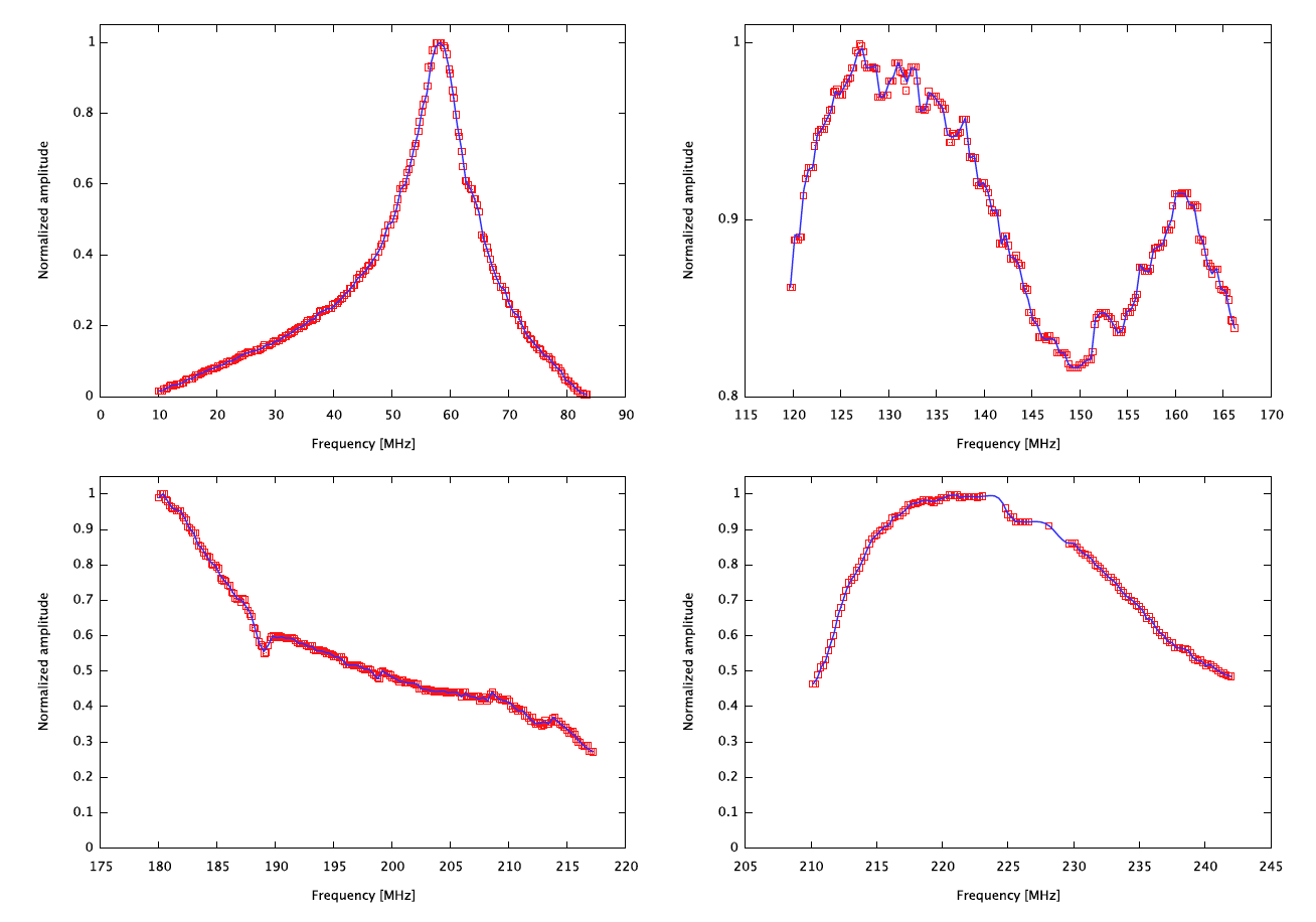
Figure 4: The bright quasar 3C196 has been observed using the core and remote stations. Observations of 3C196 between 15–78 MHz were obtained in two observing sessions (15–30 MHz in one session, and 30–78 MHz in the other). For each subband, a system gain was determined, and the gain amplitude was taken as the value of the global bandpass at the frequency of the particular subband. These figures show the normalized global bandpass for several of the LOFAR bands. The global bandpass is defined as the total system gain converting measured voltage units to flux on the sky. These bandpass measurements were determined using short observations of the bright source 3C196 and calculating the mean gain for all stations in each sub-band. The values have been corrected for the intrinsic spectrum of 3C196 assuming a spectral index of -0.70 (Scaife & Heald 2012). Curves are shown for (upper left ) LBA from 10-90 MHz with 200 MHz clock sampling, (upper right) HBA low from 110-190 MHz with 200 MHz clock sampling, (lower left)HBA mid from 170-230 MHz with 160 MHz clock sampling, and (lower right) HBA high from 210-250 MHz with 200 MHz clock sampling.

Although great care has been given to deriving the numbers in this document, still they have to be treated with some caution :

• Definite values for α₁ and α₂ have to be determined during the commissioning of LOFAR.

• The sensitivity numbers have been calculated taking a representative out of the plane value for the sky brightness. However, the sky brightness varies with factors of a few and this needs to be taken into account. Furthermore, the very bright galactic plane will contribute quite a lot of power through side and, in some cases, grating lobes increasing the effective visibility noise.

• The inner sidelobes of a (HBA) station need to be suppressed to reduce scattered sidelobe noise. This will be done by tapering the station beam which has the drawback that the sensitivity will be reduced by 30-50%. The tapering will result in a larger station beam, leading to an increase in survey speed. Note however, that tapering will always result in a loss of survey speed.

• The sensitivity of a phased array like LOFAR is less at low elevation due a number of reasons. These include (i) smaller gains of the dipoles, (ii) reduced projected collecting area of the phased array, (iii) longer paths length through the ionosphere, (iv) larger separation of the ionospheric line of sight of the calibrator sources. Considering the first two points, currently sensitivity values for a pointing at 45 degrees has been used. The latter two points imply that remaining calibration errors will be larger at low elevations.

• Related to the point above, please note that below approximately 30 degrees elevation the sensitivity drops significantly such that the Sun becomes the only viable target for interferometric observation below about 10 degrees elevation.Commissioning observations have managed successful imaging of a target at -7 degrees declination, but imaging is not straightforward and the following points need to be noted:
  • The thermal noise cannot be attained at these declinations;
  • Short baselines have to be flagged;
  • Some additional flagging of data may be required.

Furthermore, the shorter length of time that such targets are above a useable horizon can severely limit the u-v coverage attainable.  Therefore for interferometric observations, -5 degrees declination should be regarded as a lower limit and targets should preferably be above the celestial equator.  Proposers wishing to image targets below the celestial equator are expected to justify that their observing programme can attain the sensitivity and/or u-v coverage required.