Observing Strategies
LOFAR can return simple time/frequency beam-formed data instead of, or combined with, interferometric data. Array beams are calculated from the data streams from one or more stations in order to produce time-series and dynamic spectra for high time and frequency resolution applications. Typical applications include pulsars, solar and planetary studies.
The minimum integration time is 5.12 μs. The maximum spectral channel width is the width of one sub-band (195.3125 kHz with the 200 MHz clock). Sub-bands may be split into a number of channels (allowed values: 1, 8, 16, 32, 64, 128 and 256), to provide higher spectral resolution. Increasing the spectral resolution comes with a corresponding increase in the minimum integration time: This is calculated by taking the inverse of the frequency resolution. For example, if 256 channels per sub-band are specified, the minimum integration time will increase to 0.0013s.
While raw data ingest is possible, data is normally processed using the pulsar pipeline or dynamic spectrum toolkit, detailed below. We suggest to at least use the pulsar pipeline to reduce the data to 8-bit to save disk space and download time. For most science cases, 8-bit data is sufficient.
In the current implementation, there are three Beam-Formed sub-modes:
1) The Coherent Stokes (CS) sub-mode produces a coherent sum of multiple stations (also known as a “tied-array” beam) by correcting for geometrical and instrumental delays. This produces a beam with restricted field-of-view, but with the full cumulative sensitivity of the combined stations.
This sub-mode is currently restricted to observations using only core stations; stations outside the core do not use the same clock and are not fully phased-up to the core stations.
The total number of simultaneous tied-array beams that can be formed is a function of the number of stations and number of subbands used. Using 22 core stations, for the full bandwidth, we can support 3 rings with 16 channels per subband (12.2 kHz) and 8 integration steps (0.65 ms) or 200 subbands with 4 rings with 16 channels per subband (12.2 kHz) and 6 integration steps (0.49 ms). If the bandwidth is reduced, the number of tied-array beams can be increased in proportion.
2) The Incoherent Stokes (IS) sub-mode produces an incoherent combination of the various station beams by summing the powers after correction for only the geometrical delay. This produces beams with the same field-of-view as a station beam, but results in a decrease in sensitivity compared to a coherently-added tied-array beam.
One such incoherent array beam can be formed for each of the specified station beams - i.e., if all the stations being summed split their recorded bandwidth across say 8 pointing directions, then 8 incoherent array beams can be formed from these.
All LOFAR stations, including the international stations, can be summed in this sub-mode.
3) The Fly’s Eye (FE) sub-mode records the individual station beams (one or more per station) without summing. This is useful for diagnostic comparisons of the stations and other applications where station data need to remain separate. In combination with the Complex Voltage sub-mode, Fly’s Eye can be used to record the separate station voltages as input for offline processing, but be aware that the data volumes for this are large and so the number of stations which can be included in such an observation is limited by disk I/O. For example, if 400 subbands are used, maximum number of stations used is 7.
Note: Currently Cobalt cannot handle coherent/incoherent beams together with Fly's Eye. If Cobalt detects FE, it will only perform Fly's Eye and the files that are produced are the FE files, not the coherent or incoherent beams.
Polarizations:
For the different modes explained above, polarizations can be selected:
- I: Stokes I, total intensity
- IQUV: full Stokes parameters
- XXYY: the complex voltages of the two linear polarizations, which is necessary for applications such as coherent dedispersion, fast imaging, or inverting the initial poly-phase filter (which splits the data into sub-bands at station level) to achieve the maximum possible time resolution. This is not available for incoherent stokes.
Processing
Pulsar Processing
Pulsar observations may be processed via the Known Pulsar Pipeline, as given in the following schematic and described in more detail by Stappers et al. (2011). This uses standard pulsar analysis packages such as dspsr and presto.
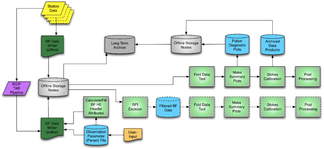
The Beam-Formed data written by the Correlator are stored on the LOFAR offline processing cluster in the HDF5 format (Hierarchical Data Format). Several conversion tools have been developed to convert these data into other formats, e.g. PSRFITS, suitable for direct input into standard pulsar data reduction packages, such as PSRCHIVE, PRESTO, and SIGPROC.
Among other things, these reduction packages allow for RFI masking, dedispersion, and searching of the data for single pulses and periodic signals. The standard pulsar pipeline can produce for example a dynamic spectrum (8-bits PSRFITS), dedispersed timeseries (32 bits PREPDATA .dat file), prepfold summaries and / or dspsr archives (.AR) files. Options can be given to select which part of the pipeline should run and with which parameters. Coherent dedispersion can be carried out online, also for multiple beams/dispersion measures.
This pipeline is only offered for use with pulsar observations.
A few standard modes exist for the complex voltage analysis:
1) The pulsar timing mode records data at 195 KHz frequency resolution from 110-188 MHz and folds the data with dspsr. The user can choose whether or not to run pdmp as part of the pulsar pipeline.
2) The pulsar scintillation mode is similar to the pulsar timing mode, but the user can choose a different frequency resolution of the output of dspsr.
3) The Fast Radio Burst mode provides a digifil data at given frequency and time integration, dedispersed to the provided dispersion measure.
4) The 8-bit data reduction mode reduces raw data to 8-bit for further analysis offline.
Note: Because of memory limitations, the standard Complex Voltage pipeline for LBA observations is not offered for observations below 30 MHz and above a DM of 40 pc cm-3, in case of a single beam. The DM limitation may be increased pending tests. When using multiple beams, or a higher DM, other frequency/DM limitations apply. Please consult the SDCO helpdesk if you want to propose such an observation.
Other Analysis Tools
Since the Beam-Formed data serve a much larger community than pulsar astronomers, a dynamic spectrum tool had been developed. This tool allows for the creation of dynamic spectra from the beam-formed data files and includes some functionality to re-bin data in time and/or frequency. It also includes the ability to only retain a useful part of the original data. Thus a user could use this tool to obtain a quick, low resolution, look at the data to identify regions of interest and then retain only these, discarding remaining, redundant, data. All dynamic spectra, whether processed or not, are stored in an HDF5 file format.
Users can request generation of quicklook plots and rebin the data using the dynamic spectrum toolkit. It is not possible to request a cut-out of part of the data, as was possible in the past. Please specify in the observing proposal that you want to use the dynamic spectrum toolkit for your analysis and to which resolution you want to rebin the data. Please also note that, currently, there are no RFI excision tools available for these data.
Performance
Processing times for typical pulsar observations are not yet robust and fully-characterised, and actual processing times can vary significantly. The following should be used to estimate processing times for the purpose of observing proposals. Not all cases are given here, so please apply a reasonable extrapolation if your particular setup is not noted. In all cases these times should apply in single- and multi-beam modes. Times are expressed in a ratio of processing/observing (P/O) times, so processing times should be calculated as this factor times the duration of the observation. The P/O is calculated from 1.2 * mean duration.
| Mode | Nr Subbands | Channels per subband | Downsampling | Nr beams | P/O | |
| HBA Stokes I | 162 | 16 | 6 | 222 | 0.9 | |
| HBA Stokes I | 162 | 16 | 6 | 1 | 0.015 | |
| HBA Stokes XXYY | 400 | 1 | 1 | 1 | 0.25 | |
| HBA Stokes IQUV | 400 | 32 | 128 | 1 | 0.03 | |
| LBA Stokes XXYY, no pdmp | 300 | 16 | 1 | 7 | 0.6 |
If you also request 8-bit conversion (XXYY mode only), please add a P/O of 0.05 per beam (e.g. Complex Voltage becomes P/O 0.3 per beam).
Sensitivity of beam formed observations
The flux that can be measured is derived from the noise level in the observation for the specific time integration and bandwidth used. See also the LOFAR imaging capabilities page for the interferometric considerations and basic station sensitivity.
SEFD (System Equivalent Flux Density): 40 kJy LBA, 3.3 kJy HBA.
Note the SEFD for LBA above 70 MHz increases up to 60 kJy at 90 MHz
Number of stations (assume 3 are missing, 21 LBA, 42 HBA_DUAL), scaling \(1 / \sqrt{N}\) [incoherent] / \(1 / \sqrt{N \times (N-1)}\) [ coherent]
Time (\(\Delta T\)), frequency integration (\(\Delta \nu\) ) : \(1 / \sqrt{\Delta T \times \Delta \nu}\)
Polarisation: \(1 / \sqrt{2}\)
For incoherent addition and flagging of data, take into account a factor 20. Higher than last cycle, as the phasing is not coherent yet and found closer to an international station.
Higher sky temperature in galactic plane: Up to a factor 15.
Theoretically, these considerations result in (for example):
- LBA with 1 hour integration time outside the galactic plane:
For a 6 MHz integration this is 38 mJy.
And for a 1 millisecond, 60 MHz integration this is 112 Jy
- HBA_DUAL
For a 1 millisecond interval this is 1.6 Jy
Please remember that a 10 sigma detection should have a flux of 10 times this noise level. Also note that a 1 hour pulsar observation that is folded into 64 bins has a basic flux level based on an integration time of 1/64 hours.