Processing, Characterization and Compression
The processing pipelines used by ASTRON are described below
Pre-processing Pipeline
Processing of the raw uv data, which consists of calibration and imaging steps, is handled offline via a series of automated pipelines.
The first standard data processing step performed by ASTRON is described below and is called the Pre-processing Pipeline:
Pre-Processing Pipeline: Flags the data in time and frequency, and optionally averages them in time, frequency, or both (the software that performs this step is labeled DP3 - the Default Pre-Processing Pipeline). This stage of the processing also includes, if requested, a subtraction of the contributions of the brightest sources in the sky (the so called "A-team": Cygnus A, Cassiopeia A, Virgo A, etc...) from the visibilities through the 'demixing' algorithm (B. van der Tol, PhD thesis). Currently, users should specify if demixing is to be used, and which sources should be demixed. Visibility averaging should be chosen to a level that reduces the data volume to a manageable level, while minimizing the effects of time and bandwidth smearing. The averaging parameters are specified by the users when they propose for an observation to be carried out.
Users willing to further process data products generated from the ASTRON pre-processing pipeline can use advanced calibration/imaging pipelines. Currently these pipelines are not (yet) offered in production. Users may download, install and run available advanced pipelines in their own computing facilities.
Computational requirements
The computational requirements of the imaging mode can be substantial and depend both on observing parameters and image characteristics.
In the following, we present practical estimates for the Processing over Observing time ratio (P/O ratio) separately for the pre-processing and the imaging steps. Note that when considering the computational requirements for the observing proposals, users should account for BOTH of these factors.
Pre-processing Time
Each of the software elements in the pre-processing pipelines has a varied and complex dependence on both the observation parameters and the cluster performance, and hence a scaling relation is difficult to determine.
To have realistic estimates of pipeline processing times, typical LBA and HBA observations with durations longer than 2 hours and adopting the full Dutch array were selected from the LOFAR pipeline archive and were statistically analyzed. The results are summarized in the following table:
|
Type |
Nr CHAN |
Nr Demixed Sources |
Nr SB | P/O |
| LBA | 64 | 0 | 244 | 0.25 |
| LBA | 64 | 2 | 244 | 0.51 |
| LBA | 64 | 0 | 80 | 0.2 [CEP2] |
| LBA | 64 | 1 | 80 | 0.3 [CEP2] |
| LBA | 64 | 2 | 80 | 1.0 [CEP2] |
| LBA | 256 | 2 | 244 | 0.72 |
| HBA | 64 | 0 | 244 | 0.81 |
| HBA | 64 | 2 | 244 | 3.0 |
| HBA | 64 | 0 | 122 | 0.9 [CEP2] |
| HBA | 64 | 1 | 122 | 1.0 [CEP2] |
| HBA | 64 | 0 | 366 | 1.4 [CEP2] |
| HBA | 64 | 1 | 392 | 2.0 |
| HBA | 64 | 0 | 380 | 1.5 [CEP2] |
| HBA | 64 | 0 | 480 | 1.4 [CEP2] |
| HBA | 256 | 2 | 244 | 4.0 |
Table 4: Pre-processing performance for >2h observations with different observation parameters and settings for demix for HBA and LBA. Although the case of 3 demixed sources has not been characterized, a large increase of the P/O ratio for both LBA and HBA is expected. Note that for setups with no CEP4 statistics, we reported the P/O values for the old CEP2 cluster: thus these values must be considered upper limits for CEP4.
These guidelines have been implemented in NorthStar, such that pipeline durations are automatically computed for the user.
Note that:
- The case of 3 demixed sources is expected to drastically increase in terms of P/O ratio for both LBA and HBA and of claimed computing resources. To safeguard the overall operations of the LOFAR system, the Radio Observatory does not support 3 demixed sources on the CEP4 cluster.
- The processing of data with resolution of 256 channels and demixed source(s) is granted based on a solid scientific justification.
Access to Data Products
All final products will be stored at the LOFAR Long Term Archive where, in the future, significant computing facilities may become available for further re-processing. Users can retrieve datasets from the LTA for reduction and analysis on their own computing resources or through the use of suitable resources on the GRID. More information are available here.
From the moment the data are made available to the users at the LTA the users will have four weeks available to check the quality of their data and report problems to the Observatory. After this time window has passed, no requests for re-observation will be considered.
DYSCO
As of 10 September 2018, all LOFAR HBA data products ingested to the Long Term Archive (LTA) will be compressed using Dysco. This decision was made after evaluating the effect of visibility compression on LOFAR measurement sets (see below for more information).
- Our tests indicate that compressing the LBA and the HBA measurement sets with dysco do not produce any visible differences in the calibrator solutions or the recovered source properties.
To process the Dysco compressed data, you will need to run the LOFAR software version 3.1 or later (built with the dysco library). The Dysco compression specifications (using 10 bits per float to compress visibility data) and the tests carried out as part of the commissioning effort are valid for any HBA imaging observation with a frequency resolution of at least four channels per subband and a time resolution of 1 second. Note that using 10 bits is a conservative choice and the compression noise should be negligible.
Need for dysco visibility compression
Modern radio interferometers like LOFAR contain a large number of baselines and record visibility data at a high time and frequency resolution resulting in significant data volumes. A typical 8-hour observing run for the LOFAR Two-metre Sky Survey (LoTSS) produces about 30~TB of preprocessed data. It is important to manage the data growth in the LTA, especially in view of the increasing observing efficiencies. One way to achieve this is to compress the recorded visibility data. Recently, Offringa (2016) proposed a new technique called Dysco to compress interferometric visibility data. The new compression technique is fast, the noise added by data compression is small (within a few per cent of the system noise in the image plane) and has the same characteristics as the normal system noise (for specific information on the compression technique, see Offringa (2016) and the casacore storage manager available here).
Commissioning tests
Before integrating the Dysco compression technique in the production pipelines, SDC operations carried out a commissioning effort to characterise how compressing visibility data using Dysco affects the calibration solutions and the images produced.
Compressing HBA data
To validate Dysco compression on LOFAR HBA data, we carried out a test observation using the standard LoTSS setup (2x244 subbands, 16 ch/sb, 1s time resolution). The raw visibilities were preprocessed (RFI flagging and averaging) using three different preprocessing pipelines: (i) standard production pipeline without any compression, (ii) enable dysco compression on visibility data, and (iii) enable dysco compression on both visibility data and visibility weights. The data products produced by the three pipeline runs were processed using the direction-independent Prefactor and direction-dependent Factor pipelines.
Comparing the gain solutions and the images produced by the prefactor and the factor runs show that compressing visibility data and visibility weights have little impact on the final output data products. The key results from this exercise can be summarized as follows:
- Compressing the measurement sets with dysco does not produce any visible differences in the calibrator gain amplitudes, clock and TEC solutions.
- Gain solutions for a given facet derived as part of the Factor direction-dependent calibration scheme are similar for a dysco compressed and uncompressed datasets (See Fig. 1).
- For one facet (containing the brightest facet calibrator), we found that the gain solutions for a few remote stations were different for the dysco compressed case (See Fig. 2). This is caused by the different clean-component models used during the facet selfcal step. However, since the image-domain comparisons are identical between different pipeline products, this is not a cause for concern.
- The mean ratio of source fluxes (see Fig. 3) between the uncompressed and the dysco compressed datasets is 1.004 +- 0.06.
- The mean positional offset in both right ascension and declination is less than 0.08 arcsec.
- For a typical LoTSS observation, the disk space occupied by the compressed visibility data is about a factor of 3.6 smaller than uncompressed data.
- Since compressing and uncompressing the visibility data is faster than the typical disk read/write times, Dysco compression does not increase the computational cost of the Radio Observatory production pipelines and the processing pipelines used by the users.
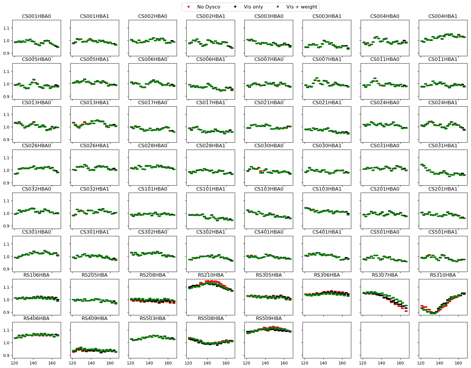
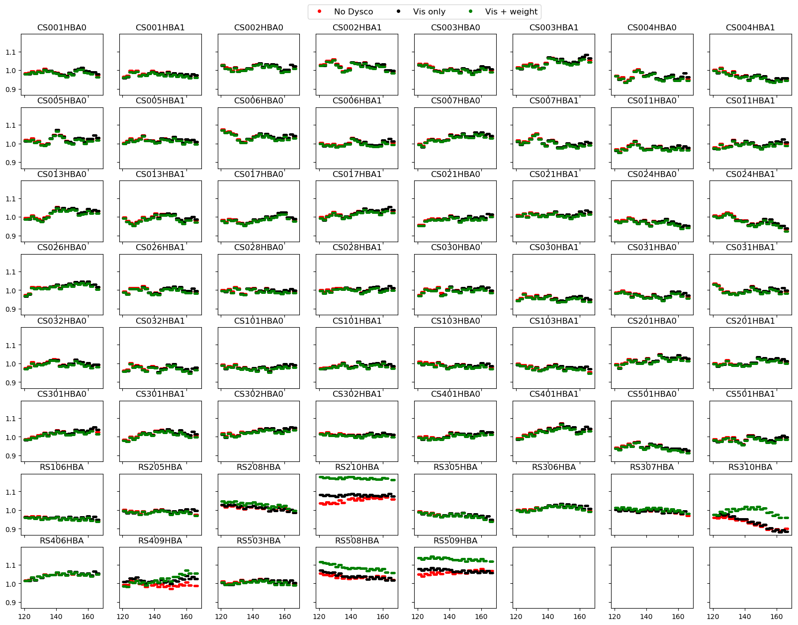 Fig 2. Plot showing gain solutions for the facet containing the brightest facet calibrator. The gain solutions for dysco compressed data is different for a few remote stations due to the difference in the clean-component model used in the facet selfcal step.
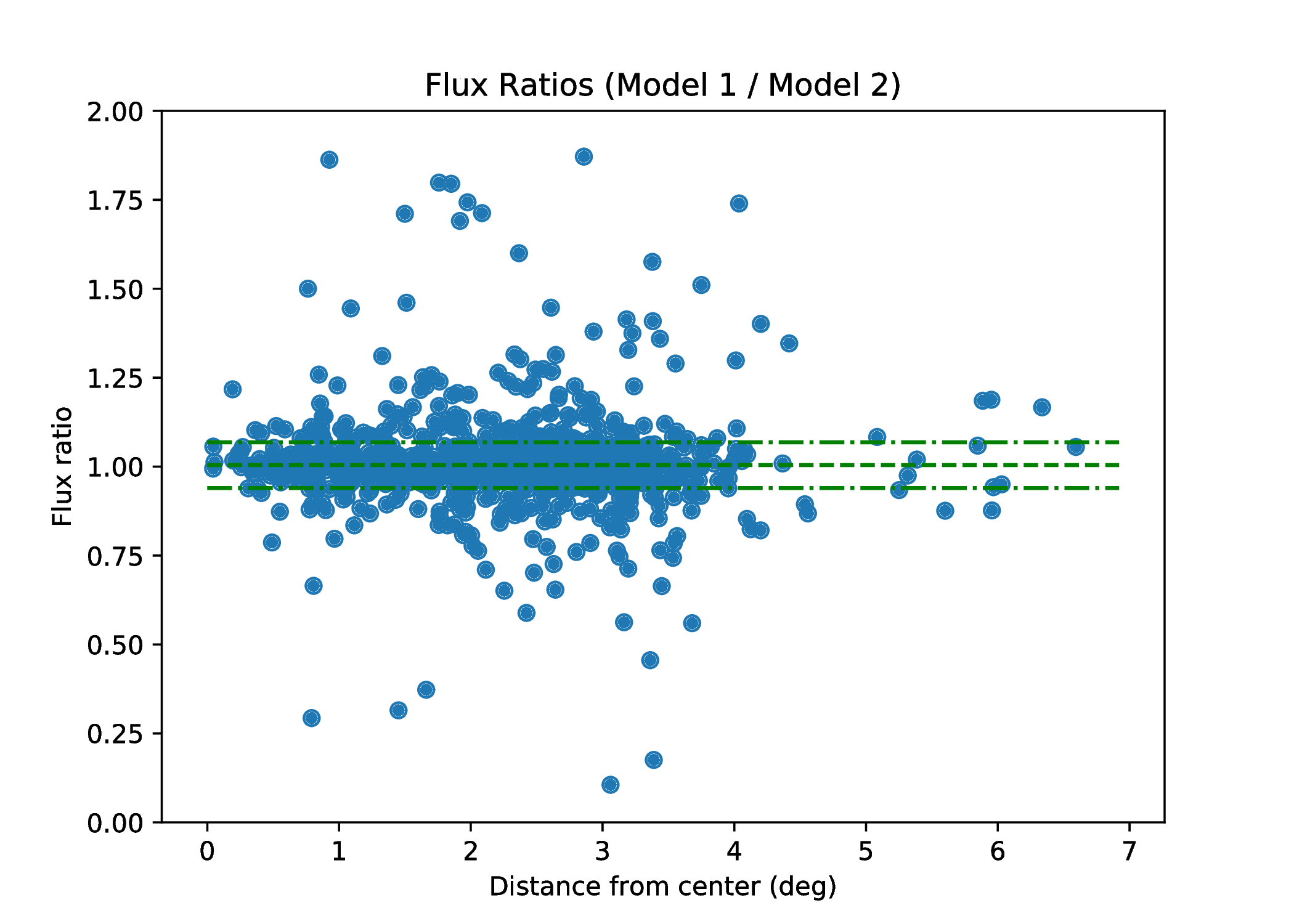
Compressing LBA data
We used an 8-hour scan on 3C 196 to validate applying dysco compression on LBA data. The observed data were preprocessed by the radio observatory with two different pipelines (i) with dysco visibility compression enables,and (ii) without dysco compression. Further processing was carried out by Francesco de Gasperin using the standard LBA calibrator pipeline. Comparing the intermediate data products produced by the pipeline, we find that dysco compression has no significant impact on the data products produced by the calibration pipeline. The key results from this exercise are listed below:
- Based on visual inspection, the calibrator solutions are identical.
- The mean ratio of source fluxes between the uncompressed and the dysco compressed datasets is 1.007.
- The largest difference in the pixel values is at the 0.01 Jy/beam level close to the bright central source (3C 196)
How do I know if my data have been compressed?
Since 10 September 2018, the radio observatory has been recording all HBA imaging observations in Dysco-compressed measurement sets. A new column has been introduced in the LTA to identify if a given data product has been compressed with Dysco. When you browse through your project on the LTA, on the page displaying the correlated data products, the new column Storage Writer identifies if your data has been compressed with Dysco. For example, Fig 4 shows the list of correlated data products for an averaging pipeline. The column Storage Writer specifies that the preprocessed data products have all been stored using the DyscoStorageManager implying that the data has been compressed with Dysco.
To process these data you will need to run the LOFAR software version 3.1 or later (built with the dysco library) so that DPPP can automatically recognise the way the visibilities have been recorded. Note that compressing already dysco-compressed visibility data will add noise to your data and hence should be avoided.
For further questions/comments, please contact SDC Operations using our JIRA helpdesk.

Calibration and Processing Tools
LOFAR Imaging Pipelines
Several imaging pipelines are available for processing LOFAR LBA and HBA data.
- LINC - Direction Independent (DI) calibration pipeline for LOFAR.
- SDCO maintains a LOFAR data reduction reference manual which contains a user guide on LINC data reduction.
- RAPTHOR- Direction Dependent (DDE) calibration pipeline for LOFAR.
- LOFAR-VLBI (long baseline LOFAR data reduction).
- Pill (pipeline for LOFAR LBA imaging data reduction - under development).
- DDFacet (direction dependent calibration software used for the LOTSS survey).
LOFAR Beam formed / pulsar tools
A GitHub repository of scripts to use for analysis of beam formed / pulsar data.
LOFAR Imaging Software (external packages)
A collection of links of documented data reduction tools developed and maintained by external experienced users.
- Dysco (a compressing storage manager for Casacore mearement sets)
- LoSoTo (LOFAR solutions tool)
- LSM Tool (LOFAR Local Sky Model Tool)
- PyBDSF (Python Blob Detector and Source Finder)
- RMextract (extract TEC, vTEC, Earthmagnetic field and Rotation Measures from GPS and WMM data for radio interferometry observations)
- Sagecal (GPU/MIC accelerated radio interferometric calibration program)
- WSClean (fast widefield interferometric imager)
LOFAR User Script Repository
A GitHub repository of 3rd party contributions for LOFAR data processing.