APERTIF DR1

APERTIF DR1

    Skip to the data access

    Go to the related publication(s)

    Introduction

    Apertif is a new phased-array feed (PAF) system installed on twelve of the fourteen dishes of the Westerbork Synthesis Radio Telescope (WSRT). Each PAF consists of 121 Vivaldi elements; the signal from these elements is combined with different weights to form forty adjacent beams across the sky, greatly increasing the field of view. Each Apertif beam is a distinct primary beam response on the sky. Throughout this documentation, an Apertif (primary) beam is sometimes referred to as a “compound beam”, emphasizing it is formed from the response of multiple individual elements.

    The imaging survey observations occur in the frequency range 1130-1430 MHz1, corresponding to a redshift of 0.26 for HI. While the lower half of this band is significantly affected by RFI, it offers a large cosmic volume for observing HI. The 24576 channels provide a frequency resolution of 12.2 kHz, or 2.6–3.2 km/s across the band for HI. The angular resolution of the imaging survey observations is ∼ 15′′×15′′/sin(δ). Imaging survey observations occur roughly four weeks out of every six weeks, with the other two weeks dedicated to time-domain surveys. The exact cadence of observations is adapted to suit maintenance and operational needs. A full description of the imaging survey observing strategy will be given in Hess et al. (in prep).

    Briefly, survey fields are observed for 11.5 hours, instead of a full 12-hour sythesis measurement, as a compromise between flexibility in scheduling and depth/maximum uv coverage. Calibrator observations alternate between a flux/bandpass calibrator (3C147 or 3C196, occasionally 3C295) and polarization calibrator (3C286 or 3C138); calibrators are observed in every Apertif beam as the different beams have different calibration solutions. Up to two survey fields can be observed in a row. Thus a survey field may be separated in time from its calibrator by ∼ 15 hours. Occasionally an observing session will start or end with a survey field in order to increase observing efficiency; then the separation in time may be longer. The calibration solutions were found to vary by less than 10% on timescales of ten days within the same beam weights model. This demonstrates that the system is stable enough to allow long periods between calibration scans with minimal impact on the absolute calibration.

    The imaging survey footprint is focused on northern extragalactic sky; Hess et al. provide a full motivation of the choice of survey regions. The imaging survey is split into two tiers: a wide-shallow tier consisting of a single observation per field and a medium-deep tier consisting of ten observations per field. Fig. 1 below shows the full four-year survey footprint in the context of local extragalactic structure; the medium-deep regions are labelled.

    Relative flux error
    Fig. 1 This figure shows a superset of Apertitf pointings (black empty circles) which are used to schedule the imaging surveys, as seen from the North Celestial Pole. Four regions of interest which will include some medium-deep pointings including Perseus-Pisces centered on Abell 272 (red); H-ATLAS (red); and HETDEX (green). Blue circles are galaxies from the 2MASS Redshift Survey between v=1000-12000 km/s which illustrate the large scale structure covered by Apertif. Orange dots are galaxies within v<550 km/s (~10 Mpc) from the Local Volume catalog by Karachentsev et all (2004). Green dots indicate the position of bandpass and polarization calibrators. Blue stars are the central positions of LOFAR deep fields.

    Observations & Processing

    Released Observations

    All raw observational data from the imaging surveys through the first year of survey observations (1 July 2019 - 30 June 2020) are released. The survey medium-deep observations during this period were focused on the Perseus-Pisces region, with an additional medium-deep field in the HETDEX region. The wide tier of the survey focused on the HETDEX region (for overlap with the LoTSS DR1), with additional coverage in the Herschel-ATLAS North Galactic Cap, and in the fall sky between 22h-0h. In total, there are 218 observations; 65 of these observations build repeated coverage of nine medium-deep fields. There are observations of 160 unique fields; with an effective field-of-view (based on spacing between fields) of 6.44 square degrees, the released observations cover just over 1000 square degrees of sky.

    Fig. 2 shows the sky coverage of released observations, with the full four-year survey footprint shown for reference. The color coding indicates the version of the pipeline used for processing (see Apercal “Versions applicable to the release” for details), where “None” means no processing was performed (see “Notes on specific observations”). “AMES” refers to observations in the medium-deep footprint, and Fig. 3 shows these repeated medium-deep fields separately as individual observations of a field may be processed by different versions of the pipeline.

    Relative flux errorFig. 2 The sky coverage of released observations, with the full four-year survey footprint shown for reference. The color coding indicates the version of the pipeline used for processing (see Apercal “Versions applicable to the release” for details).

    Relative flux errorFig. 3 A view of the processing for medium-deep fields with repeat visits. The observations are ordered in time-order and the color code refers to the same processing as for the figure above.

    Notes on the data quality/processing for specific observations can be found at Notes on specific observations.

    A machine-readable summary table of these observations can be exported using the VO infrastructure, more details are provided in section “User Interfaces”.

    Primary Beam Response

    Overview of primary beam shapes for Apertif

    Knowing the primary beam shape of a radio telescope is critical for deriving accurate fluxes away from the beam center. In the case of PAFs, the primary beam response, also known as the compound beam shape, must be independently measured for each compound beam as they are not constrained to have the same shape. Generally, formed beams further from the pointing center of the PAF will have more elongated shapes.

    Full characterization of the Apertif primary beam is ongoing work. In this documentation we describe the methods used to measure the compound beam shapes (drift scan measurements and Gaussian process regression); describe the first release of primary beam images and plans for near-term updates; and offer an initial characterization of these released primary beam images.

    We wish to emphasize that the use of the classic WSRT primary beam correction is not appropriate for Apertif. In addition to the fact that the compound beams can have non circularly symmetric shapes (see Fig. 4), the sizes of the primary beams are different from the classic WSRT. The Apertif front-ends fill the focal plane more efficiently than the old MFFE frontends, leading to a smaller primary beam shape. Fig. 5 shows one set of measured compound beam shapes divided by the classic WSRT primary beam shape. In addition to the elongated shapes (and offsets) visible in outer beams, the Apertif primary beam value is generally smaller than the classic WSRT primary beam value, confirming the smaller primary beam shape for Apertif.

    Relative flux errorFig. 4 Beam maps for all 40 apertif beams reconstructed from drift scans. Contour levels are: 0.1, 0.2, 0.4, 0.5, 0.6, 0.8. Red contours highlight the 10% and the 50% sensitivity level. These drift scans were measured in September 2019 and channel 7 corresponds to a frequency of ~ 1.363 GHz.

    Relative flux errorFig. 5 Compound beam shapes derived from drift scans divided by the classic WSRT primary beam. Contours are: 0.2, 0.4, 0.6, 0.8, 1.0.

    Drift scan method

    Beam maps are produced from drift scans performed periodically on Cygnus A (CygA hereafter). Cyg A is chosen for the drift scans since it is one of the brightest compact radio sources in the northern sky, with a brightness of 1589 Jy (Birzan et al. 2004) an extent of approximately 5′ at 1.4 GHz, which makes it an unresolved continuum source for a single WSRT dish. During the drift scan measurement the PAF is at a fixed position on the sky and Cyg A drifts through the field of view in a straight line. The separation between the drifts is 0.1 degrees in declination. This is then repeated 31 times to cover the whole field of view of the 40 Apertif beams. Fig. 6 illustrates this process.

    Drift scan observations are scheduled using the aperdrift code : https://github.com/kmhess/aperdrift

    Relative flux errorFig. 6 Illustration of drift scan observations. The dots represent the beam centres of the 40 Apertif beams, and the lines represent individual drifts across the field of view of the Apertif footprint.

    Beam models

    The auto correlation data from the drift scans is used to construct fits images of each beams response to Cyg A. Then we perform a 40 times 40 pixel spline interpolation for each beam to minimise the distorting effect of bad data (e.g. RFI) to the beam map. For this, we use the scipy package interpolate.RectBivariateSpline, which performs a bivariate spline approximation over a rectangular mesh to smooth the data.

    Once the fitting is done, we write out the resulting beam maps into a csv table and also into 9 times 40 fits files corresponding to 9 frequency bins for all 40 beams.

    We divide the 150 MHz bandwidth into 10 frequency bins when extracting the auto correlation data from the drift scans. From these we construct beam models at 9 different frequencies (chan 1-9). We do not use the first frequency bin (chan 0) because it is always badly affected by RFI.

    The code to produce the beam maps is available at: https://github.com/apertif/aperPB

    Relative flux errorFig. 7 Beam maps for all 40 apertif beams reconstructed from drift scans. Contour levels are: 0.1, 0.2, 0.4, 0.5, 0.6, 0.8. Red contours highlight the 10% and the 50% sensitivity level. These drift scans were measured in September 2019 and channel 7 corresponds to a frequency of ~ 1.363 GHz.

    Time variability

    Beam weights are measured at the start of every imaging observing run and are typically used for 2 weeks in a row. The beam weights define the shape of the compound beams. They depend on the quality of the beam weight measurement, (e.g. RFI at the time of the measurement) and also on the health of the system (e.g. broken elements on the PAFs, dysfunctional antennas). Drift scans are typically measured once per month due to the time intensive nature of the measurement. The beam models derived from drift scans observed at different times typically vary by a few percent (rms of the difference).

    Relative flux errorFig. 8 Normalised distribution of the pixel by pixel difference between beam maps observed in September 2019 and in October 2019. The rms of the distribution is 0.018.

    Beam size change with frequency

    Beam shapes and sizes change across the field of view of Apertif with the central beams being more symmetric and the beams along the edge of the field of view more elongated. Fig. 9 and Fig. 10 show the average beam size (FWHM), and the FWHM along the x and y axis as a function of beam number. Fig. 9 shows the beam size for frequency bin 7 (1.363 GHz) and Fig. 10 shows the same for frequency bin 9 (1.399 GHz).

    Relative flux errorFig. 9 FWHM as a function of beam number for channel 7 (1.363 GHz). The black line shows the average FWHM when fitting a 2D Gaussian function to the beam maps. The blue line shows the FWHM of the 2D Gaussian along the x-axis (r.a.) and the orange line shows the FWHM along the y-axis (dec). The shape of the CBs is not perfectly Gaussian, but a 2D Gaussian function is a good approximation for the beam shapes within a few percent.

    Relative flux errorFig. 10 FWHM as a function of beam number for channel 9 (1.399 GHz). The black line shows the average FWHM when fitting a 2D Gaussian function to the beam maps. The blue line shows the FWHM of the 2D Gaussian along the x-axis (r.a.) and the orange line shows the FWHM along the y-axis (dec).

    Beam sizes change linearly with frequency. The frequency dependence is on average: -2.108e-08 · freq [Hz] + 63.47. This is based on fitting a 2D Gaussian to each beam map at each frequency, taking the average FWHM from the 2D Gaussian fit and then fitting a first order polynomial to the FWHM vs. frequency for each bin. The results were then averaged for 14 different drift scan measurements. Fig. 11 shows the average beam size for each 40 beams as a function of frequency bin for a set of drift scans (grey lines). The dashed black line shows the average fitted line to the data. Some of the beams occasionally show non smooth variation with the beam size (for example beam 7, see also in Fig. 9 and Fig. 10). The cause for this in most cases is due to the effect of RFI in certain frequency bins.

    Relative flux errorFig. 11 FWHM of CBs as a function of frequency bins. We divide the 150 MHz bandwidth into 10 frequency bins when constructing the CB maps. The grey lines show the average FWHM from the 2D Gaussian fit to each CB, while the dashed black line shows the average fitted line (a and b are the parameters of the line).

    Gaussian process regression

    A second method for measuring the compound beam (CB) shapes uses a comparison of the continuum images to the public NVSS catalog and Gaussian process regression (GPR) to construct the compound beam shape.

    The Apertif images of each individual compound beam (CB) are convolved with a circular PSF of 45” to match the NVSS resolution. Then the source finding is performed, and the list is cross-matched with the NVSS catalog. After that the distribution of the relation between NVSS and Apertif total flux over a CB field of view is considered. In the absence of any biases it represents the corresponding compound beam shape.

    An example of this relation is shown in Fig. 12. The top left plot shows the distribution of 7153 sources over Beam 01 observed from August 2019 to June 2020. The size of each symbol corresponds to the fraction e.

    All the data for a given CB (40+ epochs, a few thousands cross-matched sources) is considered and the scikit gaussian_process python library is used to construct a gaussian process regression for these data. For that, the mean value is subtracted from the data. The kernel for GPR is chosen as a sum of two squared exponentials and the one representing white noise. The first kernel represents the main CB shape, and the second one represents shorter scale irregularities. After the gaussian process is trained the regression surface is obtained. The surface is then normalized to take values between 0 and 1. An example of the GPR for Beam 01 is shown in the top right panel of Fig. 12.

    With this method the “average” CB shapes over the span of all observations are obtained. We note, nowever, that the shape of a CB can change in time because of re-measurement of the beamweights, broken/repaired PAF elements, or if a particular antenna is excluded from observation.

    In order to address concerns about time-variability, the described method allows one to obtain the CB shape for a given observation, using only measurements obtained within a given beamweights set (usually a two week time span). Typically, around 500 cross-matched sources (5 - 7 observations) are needed to build the GPR accurately.

    These all-antenna CB models correspond to the middle frequency of the 150 MHz band and can be scaled further to be used for the HI or polarization cubes.

    Relative flux errorFig. 12 Top row – the total flux ratio of APERTIF to NVSS and the corresponding GPR. Bottom row – the GPR middle slices along RA and Dec.

    Released primary beam images

    The initial primary beams to accompany the first data release are those derived from the Gaussian process regression (GPR). The flux ratios between NVSS and Apertif were examined for both the compound beams derived from GPR and the drift scan methodology (see “Characterization of the primary beams”). Both sets of compound beams show similar behavior in the inner region, but the primary beam images from the drift scan methodology show systematics in the outskirts of the primary beam response, likely related to source confusion when performing the drift scans. This is under active investigation but currently only the GPR compound beam shapes are released as these appear to behave better in the outer regions.

    These primary beams are appropriate for the center frequency of the continuum images, 1361.25 MHz, over the frequency range 1292.5-1430 MHz. The drift scan measurements demonstrate the size of the compound beam changes linearly with frequency, as expected.

    The provided primary beam images are created at 100” resolution and should be regridded to match the images/cubes they are used to correct. In addition, they can be applied to other frequencies by scaling the cell size (cdelt1 and cdelt2 keywords) linearly with frequency (see subsection “Beam size change with frequency” in “Drift scan method” for the scaling) before regridding to match the data product of interest.

    Two sets of primary beam images are released for each compound beam. The first set (“orig”) is not normalized to have a peak response 1. By construction, applying these primary beam images to the Apertif data should result in measured fluxes that are consistent with those in the NVSS catalog. Note, however, that the derivation of the primary beam response images did not account for the slightly different center frequency of the Apertif continuum images (1361.25 MHz) compared to NVSS and thus there may be small changes in the flux scale due to spectral indices of sources (2% for a typical spectral index of -0.7).

    The second set (“norm”) are primary beam images normalized to have responses between 0-1, as is typical for primary beam images. Applying these primary beam images to the Apertif data will include systematic offsets between the measured Apertif fluxes and the NVSS catalog fluxes; this is discussed and quantified below in “Characterization of the primary beams”.

    Characterization of the primary beams

    In order to provide information on the reliability of the measured primary beam images, we undertake an empirical comparison to the NVSS catalog over the full data release. While similar in philosophy to the Gaussian process regression used to derive the primary beam images, this comparison provides information about overall systematics in the flux scale, in addition to quantifying the scatter in the accuracy of derived fluxes using the provided primary beam images. It also allows a direct comparison between the reliability and accuracy of primary beam images derived from different measurement techniques.

    Briefly, in order to provide a comparison over the full data release, the following steps are taken for every continuum image in the data release:

    • Convolve the Apertif continuum image to 45″ resolution
    • Regrid the primary beam image to the Apertif continuum image
    • Primary beam correct the Apertif image (mask below 10% response)
    • Create an Apertif source catalog by running pybdsf; identify sources with S/N > 5
    • Cross-match to the NVSS catalog

    The cross-matches are recorded and later combined to build a global picture of a compound beam over the full data release.

    The key value examined to understand and characterize the primary beam response images is the ratio of the Apertif integrated flux over the NVSS integrated flux. The first check was to look for systematics in this value as a function of position, since this could point to biases in the derivation of the primary beam responses. The primary beam images constructed from drift scans resulted in systematically higher flux ratios at the outskirts of the primary beam response in a consistent (south-west) direction for all compound beams. This points to an issue with source confusion around Cyg A which is under active investigation. This systematic was not seen in the primary beam images derived with the Gaussian process regression.

    The key characterization of the primary beam images is to understand the impact they have on the flux scale. Flux validation of continuum images takes an initial look at this using a single medium-deep field to look at the internal consistency of the flux scale and compare to NVSS. With the full primary beam characterization, this can be examined for each compound beam in aggregate over the full data release. While the originally returned primary beam images from the Gaussian process regression match the NVSS flux scale by construction, it is informative to undertake the comparison for the normalized primary beam images as this provides information about any overall differences in the flux scale between Apertif and NVSS (which would also be seen in primary beam images derived from the drift scan approach). Cross-matched sources were filtered to have a deconvolved major axis in the NVSS catalog < 45” and to have a measurement error on the ratio of integrated fluxes between Apertif and NVSS <0.1. Table 1 provides (as a csv file) the median ratio between the integrated fluxes, along with the standard deviation of the flux ratios and the median measurement error on the flux ratio. Table 2 provides (as a csv file) these same values but limited to the inner part of the primary beam images where the response level is ≤50%. The typical value is 1.11 in both regimes, indicating the Apertif fluxes are systematically ~10% higher than those from the NVSS catalog. The Apertif fluxes are expected to be ~2% higher based on a typical spectral index of -0.7 and the difference in center frequency in between Apertif and NVSS. In addition, the NVSS integrated fluxes are catalog flux values, corrected for various biases, while the Apertif integrated fluxes are measured directly from the images and may include calibration and clean biases. This will be examined in more detail in the forthcoming data release paper (Adams et al., in prep).

    Table 1 and 2 also include the standard deviation of the flux ratios for each compound beam. These values are rather large, typically ~16-17%. This does not indicate an uncertainty in the primary beam measurement at this level as there are several contributing factors. The typical measurement uncertainty is ~5%, and intrinsic source variability is on the order of ~10% (e.g., Hovatta 2009). The data release paper will undertake an accounting of all sources of scatter to quantify what the uncertainty on the flux scale from primary beam variability might be. In addition, the internal consistency of flux measurements for all medium-deep observations in the data release will be undertaken to provide an additional handle on the accuracy of the flux scale within the Apertif datasets.

    Table 1: Median ratio of Apertif/NVSS integrated flux, standard deviation of flux ratio, and median measurement error of flux ratio over the full Apertif primary beam (to 10% level) : Table-1-Median-ratio-of-Apertif-NVSS-integrated-flux.csv

    Table 2: Median ratio of Apertif/NVSS integrated flux, standard deviation of flux ratio, and median measurement error of flux ratio over the inner Apertif primary beam (≥50% level) : Table-2-Median-ratio-of-Apertif-NVSS-integrated-flux.csv

    Apercal

    Overview and Structure

    The Apertif calibration pipeline Apercal is a combination of different modules, which are usually executed one after another. An overview of the whole reduction pipeline is given in Fig. 13. Each rectangular box represents a single module. The grey boxes encapsulate the astronomical software packages used within the individual modules. Arrows illustrate the data and workflow within the pipeline. The dashed arrows and lines are routines which are currently in development.

    Relative flux errorFig. 13 Apercal structure diagram

    At the top level, the role of each module is:

    • AUTOCAL: The automated pipeline trigger, detecting new observations appearing in ALTA and starting a new pipeline call
    • PREPARE: Sets up the directory structure used by Apercal and retrieves data from ALTA into this structure.
    • PREFLAG: Flags the data
    • CROSSCAL: Solves for and applies the cross-calibration solutions
    • CONVERT: Converts the data from MS to miriad internal format
    • SELFCAL: Derives and applies phase and (optional) amplitude gain solutions from the target dataset
    • CONTINUUM: Produces continuum mfs images
    • LINE: Produces dirty line cubes and corresponding dirty beam cubes
    • POLARISATION: Produces Stokes V mfs images and Stokes Q & U cubes
    • MOSAIC: In progress, produces mosaics of an observation and (eventually) between observations
    • TRANSFER: Writes self-calibrated uv data to UVFITS format for archiving

    In the following, we give more details on each of the individual modules.

    Apercal pipeline modules

    AUTOCAL

    When a new observation is uploaded to the Apertif Long Term Archive (ALTA), AUTOCAL automatically retrieves information about the target, flux and polarisation calibrator and triggers the start of the pipeline. Operating as a cron job, AUTOCAL first identifies a given observation as a target and then searches the Apertif Task DataBase (ATDB) for calibrators before and after.

    Once AUTOCAL has successfully identified a target and the accompanying polarisation/flux calibrators, it sends all necessary information to Apercal, so that the pipeline can begin downloading the relevant data from ALTA. In addition to triggering the pipeline, AUTOCAL also triggers the automatic quality assessment (QA) pipeline, which inspects the raw data, calibration solutions and images, and ingests the processed data products back to ALTA, with associated notifications for each stage.

    PREPARE

    Apercal defines a directory structure for processing where each module uses its own subdirectory to access data and save outputs. All of the following modules (except CONVERT) use a single subdirectory, so that individual steps can easily be deleted and restarted. The naming of the directories can be adjusted to the needs of the users with keywords in the configuration file.

    The main tasks of the PREPARE module are the setup of the directory structure and the download of the data. Once the module is executed given an input target and calibrator datasets, it checks the availability of the data on the local disc. In case data is not locally available, the module checks the availability on ALTA via an irods framework. If successful, a python routine is used to download the data to the local disc and to place it in the appropriate position of the directory structure. After a dataset has been successfully copied from ALTA or located on disc, the correctness of the file is checked via a checksum.

    A minimum of a target dataset and a flux calibrator need to be present for this step to be successful. This condition ensures that, if no flux calibrator is available, the execution of the pipeline is stopped. On the other hand, the pipeline will continue when a polarised calibrator is not available. In this case, the polarisation calibration within the CROSSCAL module is omitted and no polarisation imaging is performed. We want to note that for pipeline runs using the automatic trigger via AUTOCAL a missing polarised calibrator is diagnosed as a failed observation and stops the pipeline.

    PREFLAG

    The PREFLAG module handles all pre-calibration flagging of the data. It can be separated into three different operations: The flagging of data with issues known a priori, additional manual flagging, and automatic flagging routines to identify and mitigate spurious radio frequency interference (RFI). The first two operations use the drive-casa python wrapper to parse commands to CASA while the last one uses the AOFlagger routines.

    The subroutines for a priori known issues cover three distinct operations: First the data is checked for shadowing effects, where the aperture of one dish is blocked by another. The next step is a mitigation of the effect of the steep bandpass edges of the individual subbands of the Apertif system. The first two and last channel of each 64 channel subband is flagged.

    Subroutines for the manual flagging step encompass the removal of auto correlations, entire antennas, specific cross-correlations, individual baselines, channel and/or time ranges. Any flagging commands not covered by the standard commands can be parsed to a file using the standard CASA-syntax. All manual flags are supposed to be used either when known elements within the Apertif system are not working or a user identifies additional issues during calibration of the data. The data ranges to flag for the above mentioned subroutines are specified in the configuration file.

    The last step of the module uses the AOFlagger (Offringa+ 2012) routines to automatically identify and flag any unknown and previously not flagged RFI in the calibrator and target datasets. A custom flagging strategy was designed which suits both, short calibrator and long target field observations.

    CROSSCAL

    During the cross calibration step, an astronomical point-like known reference source (a calibrator) is used to derive the calibration solutions, which are then transferred to an unknown target field.

    The current calibration strategy encompasses a short flux and polarisation calibrator observation in the centre of each individual beam before or after a target field observation has been executed.

    The cross-calibration step solves for the bandpass, gain, delay and polarisation leakage solutions of the flux calibrator. While the flux calibrator is unpolarised the cross-hand delay and polarisation angle solutions are derived from the polarised calibrator using the standard CASA routines. In case a polarisation calibrator has not been successfully observed or its dataset has not passed the PREFLAG module, polarisation leakage, polarisation angle and cross-hand delay solutions are not determined. Bandpass, polarisation leakage and polarisation angle solutions are derived on a per-channel basis to mitigate any effects within the observed bandwidth. For the unpolarised calibrators the flux density scale from Perley & Butler 2017 is used while for the additionally needed information for the polarised calibrators, such as the polarisation angle, degree of polarisation and Rotation Measure, Perley & Butler 2013 is used.

    Calibrator data are automatically checked for problematic dish-beam combinations. Problems here arise from individual receiver elements in the PAF, which are malfunctioning due to broken connectors, cables or electronics. These problematic beams are spotted most easily in the auto-correlation data. Currently, this is done by checking the autocorrelations of the flux calibrator after a first cross-calibration for each dish/beam combination. The currently implemented metric checks that not more than 50% of the auto-correlation data show amplitudes of more than 1500 K, which is the value, derived from our experiences, where significant artefacts in the images become apparent. In addition the bandpass phase solutions of the flux calibrator are investigated after calibration for a standard deviation higher than 15°. If one of the above mentioned criteria applies to a dish-beam combination, the specified data is marked and flagged automatically. The flags are then applied to the target and polarisation calibrator data. The criteria determining the outcome of these metrics are dependent on the quality of the input data, so that the whole cross-calibration is performed in an iterative way. A maximum of four crosscal iterations are allowed after which the CROSSCAL module gives a final result. The pipeline is stopped for beams not passing this stage. If a beam passes the checks, all available calibrator solutions are applied to the target field dataset. Any further processing of the calibrator datasets stops here and the following modules only focus on the target data.

    CONVERT

    Since MIRIAD is not able to access the Measurement Set (MS)-format native to CASA, we need to convert the file format before doing any further reduction. Unfortunately a task for a direct conversion from MS to MIRIAD format is not available, so that we have to first convert to the UV-FITS standard and from there to MIRIAD. For this purpose we use the CASA task exportuvfits followed by the MIRIAD routine fits.

    SELFCAL

    Self-calibration is a standard procedure in radio interferometric data reduction to enhance the dynamic range of images. Small changes in the processing of the signals in the receiver electronics (e.g. temperature changes) and ionospheric and tropospheric variations of the Earth’s atmosphere cause dampening of the received amplitudes and small delay variations, respectively, over the time of the target observations. These usually slowly changing variations cannot be compensated by the bracketing calibrator observations and therefore need self-calibration.

    The task of the SELFCAL module is to solve for the antenna and feed time based variations of the target data within a self-regulating algorithm using the self-calibration technique. To guarantee the stability of the self-calibration process and the processing within a reasonable time frame, several preliminary steps are executed within SELFCAL before the actual self-calibration starts.

    First, the target data is averaged down in frequency by a factor of 64 over the 64 channels of each subband resulting in a frequency resolution of 0.78 MHz to accelerate the self-calibration. We do not expect any strong amplitude or phase variations within this frequency span. It is important to note that this frequency averaged dataset is only used for continuum and polarisation imaging in later stages of the pipeline and any HI-line imaging is performed on a dataset with the original resolution where the derived self-calibration gains are interpolated and applied.

    In order to mitigate any influence of strong HI-line emission or residual RFI on the self-calibration solutions we generate an image cube out of the averaged data. For each image in the cube its standard deviation is measured. An outlier detection algorithm is used to locate the channels affected by either above mentioned reasons and flag them in the averaged dataset. As above, these flags are only used for the continuum and polarisation imaging later in the pipeline and not for HI-line imaging.

    The performance of the self-calibration is often strongly dependent on the first image passed to the solver. In order to start the self-calibration with an image of an optimal initial quality, we use the information provided by radio continuum surveys at the same wavelength. For this purpose we first query the catalogue of the Faint Images of the Radio Sky at Twenty-Centimeters (FIRST) Survey.

    Since this survey does not cover the whole Apertif survey footprint information for fields outside of the FIRST footprint are collected from the Northern Very Large Array Sky Survey (NVSS). A fractional bandwidth of ~20% is used for observations, so that we need to account for the spectral index and primary beam variations over frequency. For acquiring a spectral index for the sources in our skymodel we query the Westerbork Northern Sky Survey (WENSS) catalogue and cross-match. Since WENSS has inferior resolution compared to the other two surveys, we account for multiple source matches by summing the fluxes of the individual components to derive the spectral index and assign the same value to all for them. We then account for the primary beam response of the Apertif system by using the primary beam model of the WSRT as an approximation. The final skymodel is then generated by directly fourier transforming the catalogue source fluxes and positions into the (u,v)-domain with the MIRIAD task uvmodel. This ensures that all our images are aligned to the same common reference frame given by the above mentioned surveys. In addition the resolution of this parametric skymodel is not limited by the pixel raster of the images, but rather the fitted position of the sources. The solution interval for this parametric calibration is usually on the order of several minutes, which is set in the config file.

    The next step involves the actual self-calibration iterations. Each iteration consists of inverting the (u,v)-data using the MIRIAD task invert followed by an automatic masking routine involving the source finder PyBDSF to limit the CLEAN algorithm to islands of real emission. All self-calibration and imaging is performed on the total intensity Stokes I parameter. Image deconvolution is executed using the multi frequency CLEAN-algorithm implemented into the MIRIAD task mfclean, which uses a first order polynomial to derive the spectral index of the sources within the imaged bandwidth. After cleaning, restored and residual images are created using the task restor. The CLEAN model generated during the cleaning process is then used to derive new calibration solutions.

    The CLEAN algorithm only performs perfectly for images which only consist of point-sources and do not show any calibration artefacts. Due to these circumstances and the fact that CLEAN is an iterative non-linear process, which can diverge, adaptive thresholds need to be set and constant quality assurance performed. For each cleaning process within a self-calibration cycle three different thresholds for generating masks are calculated: the theoretical noise threshold , the noise threshold Tn and the dynamic range threshold .

    The theoretical noise T is determined by calculating the standard deviation from images generated in circular polarisation (Stokes V). Astronomical circular polarised sources are very rare on the sky and if present only at very low flux levels. Residual RFI on the other hand is often circular polarised and raises the noise levels of these images. The noise statistics of these images are therefore well representing the actual quality of the data and the theoretically reachable noise of the final images. is given in units of Jy and defined as

    where is the confidence interval for regarding islands of emission as real. This is usually set to . If at any during a CLEAN-cycle this limit is reached, the current cycle is finished and the self-calibration stops.

    In order to guarantee a smooth convergence of the self-calibration skymodel the two additional thresholds and Tn set limits for the maximum dynamic range achievable in an image without reconstruction and the adaptation to image artefacts, respectively. The dynamic range threshold within a cycle is defined by the number of the current major cycle m, the initial dynamic range and a factor defining how fast the threshold should increase such as

    where is the maximum pixel value in the residual image of the previous cycle. The parameter is dependent on the level of the first major sidelobe in the dirty beam. The ratio between the maximum and this value gives the maximum dynamic range by which an image can be cleaned before another cycle of image reconstruction needs to be performed.

    The adaption of the threshold for stopping each individual run of the CLEAN algorithm Tn is given by

    where n is the number of minor cycles and handling how aggressive the cycles are performed. For each individual run of mfclean all three thresholds are calculated and the maximum set as a limit for the generation of masks in PyBDSF. Then cleaning is performed within this mask down to a level of the mask level divided by the parameter , which is usually set to .

    The length of the solution interval s for each self-calibration cycle is determined by

    where is the total observation time, again the iteration of the current major cycle and

    where is the number of clean components, the flux of each individual clean component, SNR the needed signal-to-noise ratio, the theoretical noise, the number of baselines, the number of solution intervals over frequency and the number of polarisations to solve for. SNR is set to 3 for phase-only calibration and to 10 for combined amplitude and phase calibration. These arithmetics ensure that solution intervals decrease during the self-calibration process consecutively while still containing enough signal-to-noise for a proper calibration.

    The SELFCAL module first performs up to a given maximum number of iterations of phase-only self-calibration. Then it decides on the amount of flux and therefore the available SNR if and with which solution interval combined amplitude and phase self-calibration is executed. If at any point during the process the theoretical noise limit is reached, SELFCAL performs only one last iteration of self-calibration.

    To improve the stability of the pipeline and the quality of the calibration solutions several metrics for quality assurance were implemented. At the beginning of each cycle, a multi-frequency image of circular polarisation (Stokes V) is generated. Since the circular polarised sky is essentially empty any sources in such an image would hint to severe calibration problems. Therefore, the image statistics can be analysed for following a normal distribution resembling Gaussian noise. This was implemented using the skewness and kurtosis of the distribution. If these values exceed a certain number given in the config-file, the self-calibration is aborted.

    During and after each imaging and cleaning cycle the dirty image, the cleaning mask, the clean component model image and the restored images are checked for any obvious problems resulting from a divergence of the calibration routines. The maximum value in dirty images of total intensity should always exceed the minimum. In addition, no Not a Number (NaN)-values are expected in the image. Both conditions are checked when starting a cleaning where new solutions were derived and applied to the data and a new dirty image is generated. Masks are checked every time for containing any CLEAN components at all. The clean component image is checked for clean components with unrealistically strong negative or positive fluxes. The restored image is again checked for containing no NaN-values and for strong positive or negative values. The final residual image should mostly consist of noise and is therefore checked for gaussianity.

    A combined amplitude and phase calibration (A&P) is not as stable as a phase-only calibration due to the increased degrees of freedom, so that this step can easily worsen the image quality due to diverging calibration solutions. Therefore, in addition to the quality assurance process described above, we added an additional metric to check the quality of the A&P calibration compared to the phase-only one. After the A&P calibration we generate another dirty image and compare the image statistics independently, namely its maximum, minimum and standard deviation with the dirty image of the last phase-only self-calibration cycle. If the ratio of one of those values exceeds a limit given in the config-file the A&P calibration is assessed as failed and any following module will use the last successful phase-only self-calibration solutions. Calibration solutions are applied in the subsequent modules before any further imaging is performed.

    CONTINUUM

    The CONTINUUM module performs two different tasks to generate final deep continuum Stokes I images. First it generates a deep multi-frequency image using the mfclean task in MIRIAD and secondly several individual images spanning narrower frequency ranges over the full bandwidth using the task clean are produced. The purpose of this is to generate an as deep as possible total intensity image with the maximum possible resolution (given by the highest frequency) and in addition derive reliable spectral indices and curvatures for as many sources as possible. In fact multi-frequency cleaning generates these images already, but their values are only reliable in cases of high signal-to-noise ratios. For both imaging steps we use a uniform weighting to acquire the maximum possible resolution on the order of 12’’. Images usually have a size of 3073x3073 pixels with a pixel size of 4 arcseconds, which allows the imaging and cleaning of any sources up to the first sidelobe level of the primary beam response in order to minimise artefacts.

    Cleaning and masking iterations are in both cases continued until the theoretical noise limit has been reached. Masking and validation of all continuum images is performed in the same way as described for the SELFCAL module.

    LINE

    The LINE module first applies the derived self-calibration solutions to the non-averaged data. This is performed using the MIRIAD task gpcopy. It automatically takes care of the different frequency resolution of the two datasets by interpolation.

    The HI-line imaging is the most computing intensive task in the Apertif data reduction, so that several endeavours have been undertaken to optimise its performance. For a better handling of the data and the image cubes imaging is performed by generating eight individual cubes over the 300 MHz of bandwidth with a small amount of overlap in frequency. The overlap is necessary to avoid splitting the detected line emission of individual objects between two adjacent image cubes. In order to improve sensitivity and save processing time and disc space, data between 1130 MHz and 1416 MHz are averaged in frequency by binning three channels together. The data at the highest frequencies which features the Galactic neutral hydrogen and small galaxies in the nearby Universe retains its full spectral resolution of 12.2 kHz.

    In order to generate image cubes containing only HI-line emission the continuum has to be subtracted. Several different approaches are possible here: the fitting of baselines to the amplitude of the data followed by subtraction, the subtraction of constant fluxes over frequency in the image domain and the direct subtraction of a continuum clean component model from the (u,v)-data. The best performance in terms of time consumption was achieved with the latter method, so that we decided to use this in Apercal. For this subtraction the final clean model of the CONTINUUM module is used.

    Finally the actual images are produced. MIRIAD does not account for the position dependence of sources situated outside of the pointing centre for large fractional bandwidth, if executed in line imaging mode. Therefore, we have to generate an image for each individual frequency and combine the final images into a cube. Since imaging of individual channels is very computing intensive, but also the imaging process for each individual channel is independent from another we optimised this step by implementing an OpenMP support with the python pymp library .

    ..[2] https://github.com/classner/pymp

    POLARISATION

    Polarisation imaging is performed in Stokes Q, U and V. Q and U fluxes from astronomical sources exhibit a sinusoidal dependence of the square of the observed wavelength. In addition, Stokes Q, U and V fluxes can have negative values in contrast to Stokes I, which needs to be positive in all cases. These effects would lead to bandwidth depolarisation in case of multi-frequency imaging of Stokes Q and U over our full 300 MHz bandwidth. Therefore, we image Stokes Q and U as cubes, using the same method as described for the LINE module, where one image is generated for a bandwidth of 6.25 MHz. This mitigates the effect of bandwidth depolarisation for most astronomical sources. In addition, this method allows the usage of the Rotation Measure Synthesis technique in post-processing, so that the linear polarisation properties of the detected sources can be analysed in more detail than with the standard methods, which suffers from bandwidth depolarisation effects. Typical reachable Faraday Depth are still on the oder of several thousands, so that the polarised emission of nearly all astronomical sources is still recoverable with these specifications. Spatial resolution of the Stokes Q and U cubes is slightly lower (on the order of 15 arcseconds) in comparison to the continuum images.

    Stokes V is representing the circular polarisation, which does not show any sinusoidal behaviour. Due to this fact and since the circular polarised sky is very faint, we perform a multi-frequency synthesis for imaging Stokes V. This also allows to maximise the sensitivity of the produced images to detect possible circular polarised sources.

    For all polarisation images cleaning is performed using the final mask generated by the multi-frequency imaging part of the CONTINUUM module. Since polarisation images usually only show very faint emission, the clean threshold is set by the standard deviation of the pixels in the image. This accounts, especially for the Stokes Q and U images, for the variations of the noise over the imaged bandwidth. For cleaning Stokes Q and U we used the MIRIAD task clean and for Stokes V mfclean.

    MOSAIC

    Currently we are not producing mosaics of the calibrated data during Apercal runs for the data release, but for reasons of completeness we explain the currently available mosaicking routines in the following. The mosaicking routines are independently implemented in order to address features specific to Apertif, namely varying primary beam responses for the different beams (see “Overview of primary beam shapes for Apertif”) and the ability to include correlated noise.

    Once all data of an observation have been processed through the CONTINUUM, LINE and POLARISATION modules, the MOSAIC module is executed to generate a combined image of all beams of one observation taking into account the response of each compound beam. Images are regridded to a common grid centred on the central beam of the observation and then corrected for the Apertif compound beam response. The compound beam response has been characterised using drift scans of a strong astronomical source over the whole field of view of the Apertif Phased Array Feed (see Compound beam shape section). The different beams of one observation have slightly varying synthesised beam sizes due to different flagging of the data, so that all input images are convolved to the largest common beam.

    The combination of the input images then follows an inverse square weighting based on the compound beam response and the background noise of the individual images. The background noise is estimated using the MIRIAD task sigest, which minimises the contribution of sources for the determination of the noise level.

    Since all data of one observation has been taken using the same electronics, a correlation between the noise of different beams exists, which raises the noise level of the final mosaic. An option for including this correlation matrix during mosacking is implemented and will be used once the coefficients have been measured. First tests showed a minor change of the noise levels between correlated and uncorrelated data of adjacent beams of ~2%.

    The MOSAIC module is currently only producing continuum mosaics using the central frequency of the observational setup for correcting the primary beam response. Additional features in the future include the implementation of the frequency and long-term time dependence of the beam pattern and the combination of images of different observations. The current implementation takes approximately an hour for generating a continuum mosaic. Future improvements will include enhancements to the speed of the module, which will then allow us to generate polarisation and line mosaics within an acceptable amount of time.

    TRANSFER

    This module converts the self-calibrated MIRIAD data to more standard UVFITS format. Similar to LINE it applies the phase and, if available, amplitude self-calibration solutions to the non-averaged cross-calibrated data automatically before conversion. The calibrated visibility data, along with calibration tables and fits images/cubes, are then ready for archive ingest.

    Versions applicable to data release

    During the course of survey operations, improvements were made to the Apercal pipeline in addition to bug fixes. The table of released observations contains the specific Apercal version (including github hashtag) used for the processing of that dataset. In addition, we assign “friendly” names that encompass the main changes from a data quality point of view. These versions are described below, in chronological order:

    • Apercal_300 (300 MHz):Survey observations at the start of the survey period were processed with the full 300 MHz of data. Flagging all RFI present at low frequencies is a challenge and unflagged RFI affected the calibration of the whole band. Data processed with the full 300 MHz were not ingested. However, the raw observational data that was processed in this mode falls under the data release.
    • Apercal_150 (150 MHz):Starting with observations in August 2019, only the top 150 MHz (1280-1430 MHz) of the Apertif band, which is relatively RFI free, was processed. This resulted in a strong increase of data quality for the final data products, and thus data processed in this mode of the pipeline is considered for release. Note that the frequency range 1280-1292.5 MHz is automatically flagged as part of this pipeline version as it is heavily impacted by RFI.
    • Apercal_150_ACF (Auto-correlation flagging):

      Internal quality assessment checks the auto-correlations of dishes. High auto-correlation values indicate a dish where the formed compound beam suffers from quality issues; these data are flagged as they contribute to direction-dependent errors in final images. The cross-calibration is then rerun.

    • Apercal_150_ACF_C-D (RTC-RTD flagging):

      The RTC-RTD baseline has an elevated (noise) response level, related to the introduction of the synch-optics boards (see System notes). In order to avoid bias in the calibration / flux scale, this baseline is flagged.

    • Apercal_150_ACF_C-D_BPF (Bandpass-phase flagging):

      An additional internal QA check; if the phases of the bandpass solution have too large a rms, that dish is flagged and the cross-calibration is carried out again.

    Known issues/Caveats to the user

    System notes

    The Apertif system has not been static since the start of science operations. Small but significant changes to the system to increase stability and data quality have occurred.

    One of the biggest impacts on the final quality of images is the presence of direction dependent errors, which can be attributed to antenna elements within the PAF for specific telescopes which are malfunctioning or missing from the signal chain. Another cause of direction dependent errors is due to pointing offsets of one or more telescopes. Generally, the emphasis of system changes has been on improving the quality of the formed compound beams and pointing stability.

    The most significant upgrades to the system are listed below in chronological order:

    • Synch-optics boards on RTC and RTD:On 3 September 2019 and 5 August 2019, synch-optics boards were installed on dishes RTC and RTD. These two dishes are furthest from the control building. They were suffering from delay issues; due to jumps in interpreting the clock signal, the residual delays for these dishes would change by up to hundreds of nanoseconds, happening at random times during observations. The synch-optics boards stabilized the clock signal, preventing the very large residual delay that would lead to the loss of usable data from the dishes.
    • Targeted maintenance of individual elements:The Apertif PAF is relatively sparsely filled. Thus, any given compound beam relies predominantly on 1-2 elements. If those elements are missing from the signal chain, that compound beam will have a non-ideal shape. When in a compound beam of on one dish, the signal of a key element is missing, this presents an odd response compared to that compound beam on all other dishes. The resulting images for that beam have strong direction dependent errors. Since October 2019, the performance and gains of individual elements are closely monitored so that they can be repaired in the most expedient manner possible.
    • Attenuation tuning of individual elements:After a major maintenance, the single antenna elements need to be tuned to the nominal receiving power. If elements lie outside the accepted range of parameters, they are ignored during the calculation of the beamweights. The attenuation tuning algorithm was significantly improved starting 1 October 2019.
    • Improved beam weights calculation:The beam weight measurements used to calibrate the PAF are single-dish measurements and hence heavily affected by RFI. An improved method for identifying subbands affected by RFI was implemented on 10 December 2019. This allows beam weight values that are affected by RFI to be interpolated from nearby subbands that are RFI-free, resulting in higher quality beamweights (especially at lower frequencies) which leads to an improved sensitivity of the system.
    • Updated pointing model:On 11 December 2019 and on 11 June 2020, the pointing model for the dishes was updated. This corrects for pointing offsets caused by changes in the mechanical structure and physical pointing of the dishes.

    Other general caveats:

    • Ghosts:Channels 16 and 48 of each subband have a “ghost”; bad signal in these channels cause a false source to appear at the center of images. Thus, any source identified at the exact center of a pointing should be treated with extreme caution.
    • Aliasing:The coarse channelization of the data into subbands uses a filter that does not have a perfectly sharp frequency response. This results in some overlap of response between adjacent subbands. This effect is strongest for channels near a subband edge and also results in a sharp drop in overall response for channels at the subband edges, namely channels 0, 1 and 63 of every subband. Currently, no correction is done for the aliasing. A brute force approach is used to deal with the suppressed signal at the edges of the subbands – the low signal channels are flagged. An offline anti-aliasing filter is under development; when it is available, aliased signals will be removed, and the sharp drop in subband response will be evened out. Until then, we note that aliased signal may occur in the presence of strong HI emission and that 3/64 channels are flagged at full spectral resolution. The impact of this flagging on the spectrally-averaged line cubes is described in the “External comparison” section of the HI validation.
    • Telescope specific issues:Due to operational needs (exceptional maintenance) or because of failures (the above mentioned high residual delay issue, tracking issues, extreme RFIs, etc), one or more telescopes could be missing from an observation. Information about specific observations can be found in “Notes on specific observations” below.

    Notes on specific observations

    This section provides brief notes on observations that had observational or processing issues. This list is not exhaustive, and the user is always encouraged to examine the data and inspection plots closely.

    Observations with no released processed data

    Some observations have no released processed data associated with them. This can either be because they were processed with the 300 MHz version of the pipeline, which produced lower quality data products, or because the automatic identification of calibrators by AUTOCAL (see “Apercal overview”) and subsequent processing failed. In addition, there is a set of observations that were scheduled without RTC & RTD, thus failing to be validated for release since they did not meet the minimum resolution requirement.

    Early processing

    The following observations have no released processed data products because they were processed with the 300 MHz version of the pipeline, which did not produce data products of the required quality.

    Observations processed with 300 MHz version of pipeline.

    190711169 S2152+4114
    190712041 M1403+5324
    190713001 M0155+3130
    190713042 S2323+2904
    190714041 S1444+5058
    190718124 S2146+4340
    190719041 S1242+5058
    190719042 M0155+3130
    190720041 S2336+2904
    190721041 S1426+5058
    190722001 M0208+3130
    190725041 S1236+6041
    190725042 M0155+3130
    190726041 S2319+3130
    190727041 S1439+5324
    190727042 M0208+3356
    Autocal failures

    The following observations have no ingested processed data products because the automatic running of the pipeline failed in their case. Generally this was because of an issue with identifying calibrators. These observations can be manually reprocessed. Access to the raw data can be requested via the helpdesk.

    Observations not processed due to failure of automatic calibration identification. Notes: *Observations 028-033 failed. **Go backwards for a pol cal that has C/D (see Obs fails below).

    190728041 S2258+2904 3C147: 190727 001-040 3C286: 190728 001-040
    190731125 S2227+3130 3C147: 190801 001-040* 3C286: 190731 085-124
    190806345 S2311+2904 3C147: 190807 001 - 040 3C286: 190808 001-040
    200429042 S1446+3848 3C147: 200429 002 - 041 3C138: 200428 001 - 040**
    Observational failures

    If RTC and RTD are unavailable, an observation is considered failed. Some of the early observations from July, which don’t have processed data available, may suffer from this as both RTC and RTD had issues with delay jumps (see System notes). In addition, there are a series of observations from April/May which were inadvertently scheduled without RTC and RTD and thus don’t have processed data which passes validation. These observations are:

    Observations scheduled without RTC & RTD.

    200430053 S1131+6041
    200501001 S2346+5324
    200501042 S2346+5324
    200502054 S1142+5550
    200503001 S2358+4832
    200503042 S1443+3622
    200505016 S0001+4606
    200505057 S1446+3848
    Partially processed observations
    Calibrator identification issues

    Two observations, 191207034 and 191207035, do not have processed data products for the first seven beams, as those beams (due to scheduling complications) were not properly identified by AUTOCAL. Given the small number of beams missing, they were not reprocessed. These observations can be manually reprocessed. Access to the raw data can be requested via the helpdesk.

    Reprocessed observations
    Reprocessed with manual flags

    As part of the data release, observations where essentially all beams failed validation (e.g., four or fewer beams passed) were visually inspected to identify the cause. In some cases there were no obvious causes, other than bright sources in the field. In other cases, inspection revealed an antenna was off-source (e.g., stuck) during the observation or part of the observation occurred while the target field was not visible. In order to increase the quality of the processed data from these fields, they were manually reprocessed with the additional, visually identified, flags applied. Other fields may also benefit from individual flags and reprocessing.

    These observations are:

    Reprocessed with correct polarization calibrator

    There were two observations where AUTOCAL incorrectly assigned the same flux calibrator to be both the flux and polarization calibrator to the initial call of Apercal. These observations were reprocessed with the correct polarization calibrator.

    Observations manually reprocessed with correct polarization calibrator.

    200126082 S1428+5815 3C147: 200126 042 - 081 3C286: 200126 001 - 040
    200406054 S1611+5324 3C147: 200406 014 - 053 3C286: 200405002 - 612
    Data quality notes
    Problems with polarization data

    There is one dataset which has no polarized data products as a polarized calibrator was not able to be observed in the same observational setup. This is ObsID 200309042, field S1042+5324.

    In addition, the observation 200505057 was processed without a polarization calibrator. However, since it has no released processed data due to missing RTC and RTD and thus failing resolution requirements, it was not reprocessed. These observations can be manually reprocessed. Access to the raw data can be requested via the helpdesk.

    Data Quality

    Continuum image quality

    All released continuum multi-frequency synthesis images have passed validation, ensuring that they meet the resolution requirements, minimum sensitivity requirements, and have no significant image artifacts, as described in “Validation of processed data products: Continuum”.

    The noise values for all released continuum images are shown in Fig. 14. The left panel shows the noise distribution on the inner part of image (inner hereafter) where many sources are detected. On the right panel the noise of the outer part (outer hereafter), which is typically source-free, is considered (see “Validation of processed data products: Continuum” for more details). The median values (41.4 and 36.1 uJy, respectively) are indicated by the solid lines. The dashed lines and numbers in parentheses indicate the noise values that bound 68% of all values around the median. The median value of the inner noise is slightly larger; this is because the inner part of the image has sources and may still have minor artifacts. The outer noise represents the theoretical best that can be achieved with perfect imaging. The median outer noise is 36.1 microJy/beam and the best achievable (5th percentile) is 29.3 microJy per beam.

    The noise values skew to higher values from the median. This is likely because some images may still have minor imaging artifacts. Any issue affecting image quality will only ever increase the noise of an image.

    Relative flux error

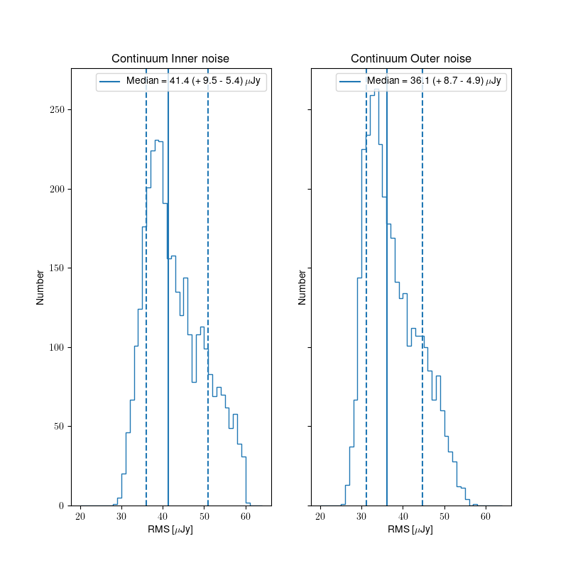
    Fig. 14 Noise distribution for all relased images in the inner (left) and outer (right) part of the continuum images.

    Polarization data quality

    All processed data products are released based on the continuum validation (see “Released processed data products”). Thus, some polarization images and cubes may be released that do not pass their own validation. However, this is a small number of images/cubes and they may still be useful (see “Validation of processed data products: Polarization” for more details).

    Fig. 15 shows the distribution of inner and outer noise for the Stokes V mfs images. Both all released images (3374) and only those that pass validation (3198) are shown. Very few polarization images fail the polarization validation after passing the continuum validation. This is to be expected as the validation criteria are very similar and the continuum and Stokes V mfs images should generally have similar quality to each other. There is no appreciable difference in the noise distribution between all released images and those that pass validation.

    The same qualitative trends are present as for the continuum noise; the outer noise is lower than the inner, and the distribution of noise values is skewed to higher noise values, due to the presence of low level artifacts that increase the noise. Overall, the noise in the polarization images is lower than the continuum; this is likely because the Stokes V images are essentially empty.

    Relative flux error

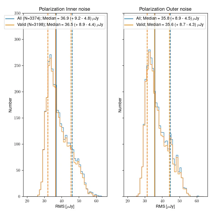
    Fig. 15 Noise distribution for all relased (blue) and valid (orange) Stokes V multi frequency images, in the case of the inner (left) and outer (right) part.

    Line data Quality

    Line cubes are released for a beam if the continuum image passes validation; thus some of the line cubes may fail their validation. The line cubes are classified as “good”, “okay” or “bad” depending on the severity of the artefacts in the line data, as detailed in “Validation of processed data products: HI”.

    Fig. 16 shows the distribution of noise for cubes 0, 1 and 2. All released cubes are shown, plus split separately into the good, okay, bad categories. The median noise over all released cubes is 1.62 mJy/bm. The median noise decreases slightly as the cubes increase in frequency; this is consistent with the RFI environment being worse at lower frequencies. As is to be expected, the median noise for good cubes is better than for the okay cubes, which are better than the bad cubes. The best achievable noise (5th percentile, cube 2, only good) is 1.32 mJy/beam.

    As with the continuum and polarization noise distributions, the distribution has a longer tail to higher noise values; this is because image artifacts and bad frequency ranges will only ever increase the noise.

    Relative flux error

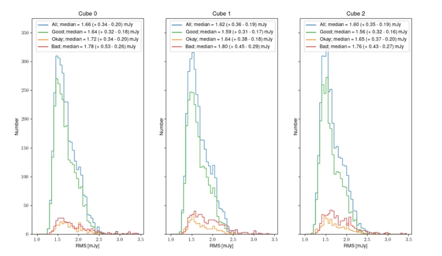
    Fig. 16 Noise distribution for all relased (blue), Good (green), Okay (orange) and bad (red) HI line cubes for cube 0, 1 and 2.

    Data quality per compound beam

    The above views of data quality combine all released observations, across different compound beams. However, the behavior of different compound beams is not identical. Specifically, the outer compound beams illuminate the edge of the field of view and thus may be expected to have a reduced sensitivity. For reference, Fig. 17 shows the compound beam layout, with colors indicating the expected sensitivity based on the forward gain of an Apertif phased-array feed (PAF).

    Fig. 18 shows the normalized average noise (over all continuum images) in the compound beam layout. The beams on the edge of layout have higher average noise values, consistent with the picture that the overall sensitivity falls off. Fig. 19 quantifies this by showing the normalized noise as a function of distance from the pointing center of the PAF; the increased noise values track with distance.

    Relative flux error

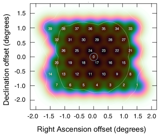
    Fig. 17 The compound beam layout for Apertif. Blue is at about the 50% level; transition between black/brown to green is at about the 85% level.

    Relative flux error
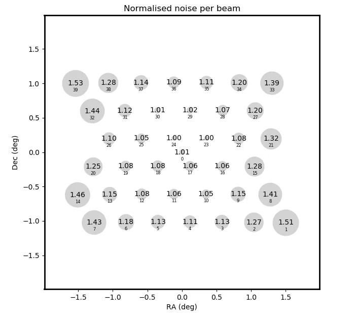
Fig. 18 The normalized average continuum noise per compound beam, shown in the compound beam layout. Compound beams closer to the edge have larger average noise values.

    Relative flux error
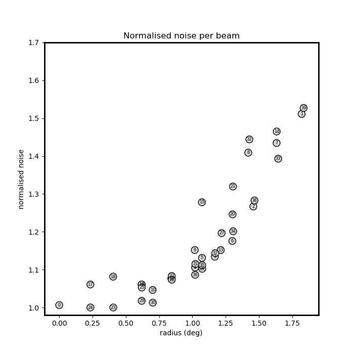
Fig. 19 The normalized continuum noise of each compound beam (labeled points) as a function of distance from pointing center of the PAF. The pattern of increased noise scales with distance from center of the PAF.

    Released processed data products

    The processed data products are of the most immediate scientific interest. Only processed data products which pass validation are considered for release. Specifically, we require the continuum multi-frequency synthesis (mfs) image to pass the validation outlined in “Validation of processed data products: Continuum”. In that case, all processed data products are released for that beam of a given observation. It may be the case that the polarization or line products do not pass their validation (see respective sections in “Validation of processed data products”). In this case, these data products are flagged in the quality assessment columns of the VO tables (see User Interfaces).

    The sections below provide a brief look at the released data products for continuum, polarization and line. The separate section “Data quality” provides a view of the data quality of these released data products.

    Released continuum data products

    The main continuum data product is the multi-frequency synthesis continuum image. The resolution is better than 15′′×15′′/sin(δ) (requirement of validation). The median noise value is ~40 uJy/beam.

    The table containing all observation / beam combinations that pass continuum validation, along with all the metrics used in continuum validation (described in ”Validation of processed data products: Continuum ”) can be exported using the VO infrastructure, more details are provided in section “User Interfaces”.

    Relative flux error

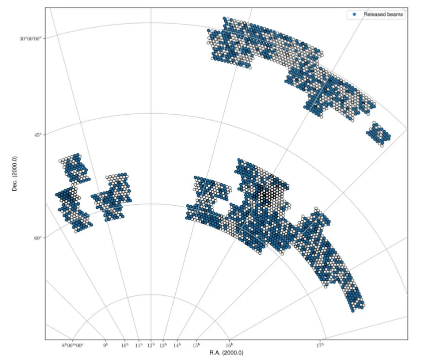
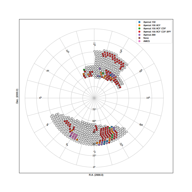
    Fig. 20 The spring sky coverage of released beams based on the continuum validation.

    Relative flux error

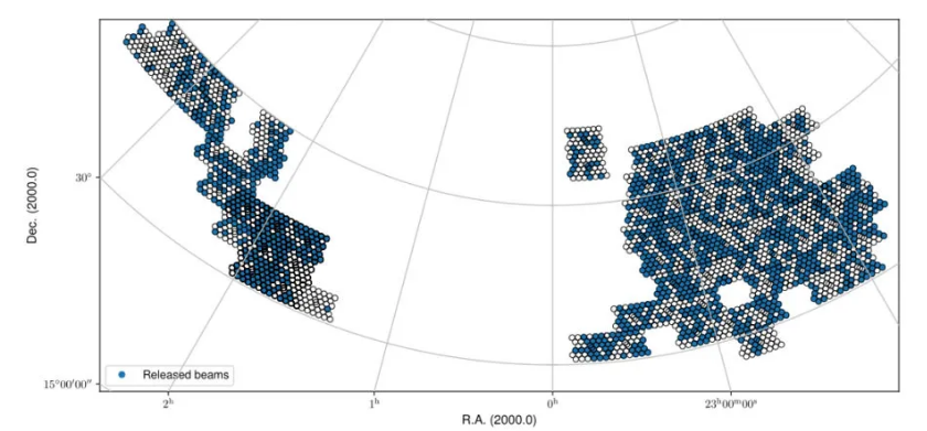
    Fig. 21 The fall sky coverage of released beams based on the continuum validation.

    Released polarization data products

    The polarized data products include a Stokes V multi-frequency synthesis image and Stokes Q&U cubes. The polarized data products are only released if the continuum validation is passed but the polarization products may not pass their own validation (see section “Validation of processed data products: Polarization”). The Stokes V images and Q/U cubes are validated separately, and their validation state is clearly given in the User Interfaces.

    A table of all released beams with the line validation status (“G”ood, “O”kay, or “B”ad) for cubes 0-2 (given by the columns “cube?_qual”), plus the metrics used for the line validation (described in HI validation) can be exported using the VO infrastructure, more details are provided in section “User Interfaces”.

    Relative flux error

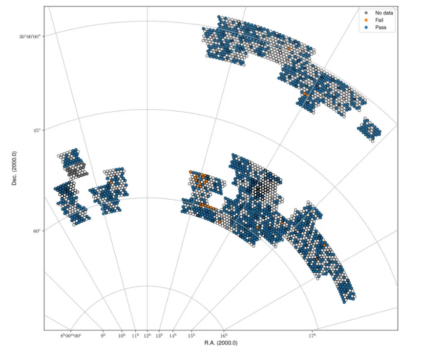
    Fig. 22 Spring sky view of the released QU cubes, color-coded by whether they pass validation or not.

    Relative flux error

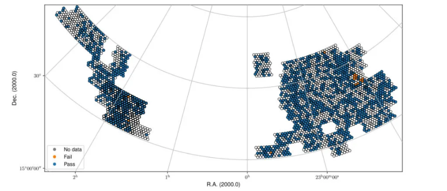
    Fig. 23 Fall sky view of the released QU cubes, color-coded by whether they pass validation or not.

    Relative flux error

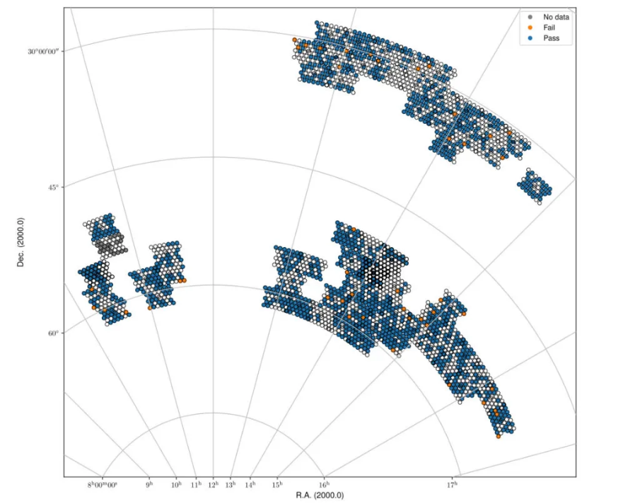
    Fig. 24 Spring sky view of the released Stokes V mfs images, color-coded by whether they pass validation or not.

    Relative flux error

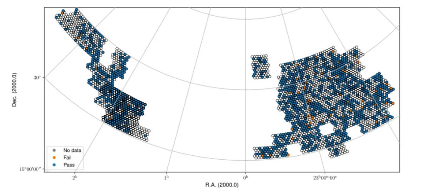
    Fig. 25 Fall sky view of the released Stokes V mfs images, color-coded by whether they pass validation or not.

    Released line data products

    The released line data products include four dirty cubes and their associated dirty beam cubes. The three lowest frequency cubes (spectrally averaged by 3 channels) are validated independently, while the highest frequency, non-averaged cube (cube3) is not directly validated but generally follows the quality of the closest cube in frequency (cube2). The details of the validation are in “Validation of processed data products: HI”.

    Table of all released beams with the line validation status (“G”ood, “O”kay, “B”ad, or “N”o cube) for cubes 0-2 (cube?_qual) plus the metrics used for the line validation (described in HI validation) can be exported using the VO infrastructure, more details are provided in section “User Interfaces”.

    Relative flux error

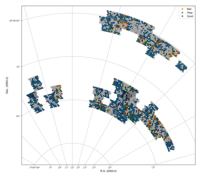
    Fig. 26 Spring sky view of the released data for cube2, color-coded by status (Good, Okay, Bad).

    Relative flux error

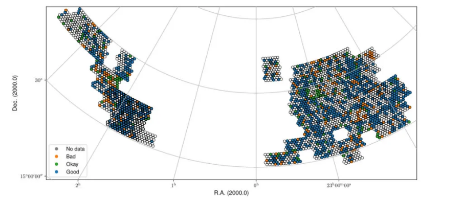
    Fig. 27 Fall sky view of the released data for cube2, color-coded by status (Good, Okay, Bad).

    Relative flux error

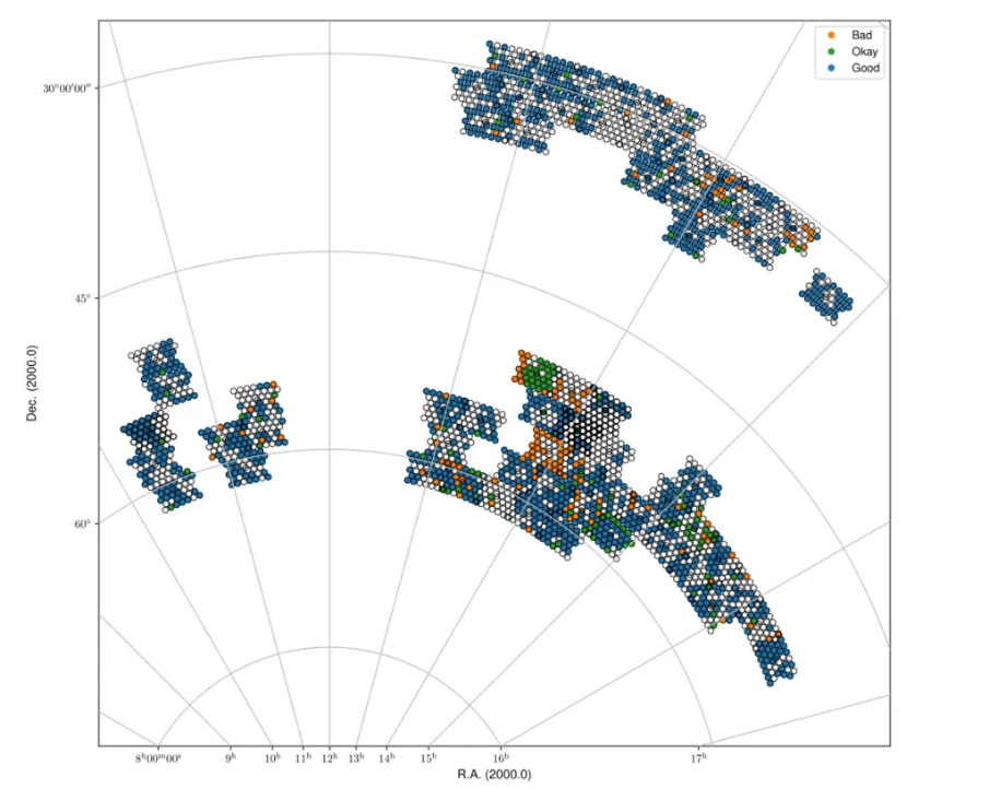
    Fig. 28 Spring sky view of the released data for cube1, color-coded by status (Good, Okay, Bad).

    Relative flux error

    Fig. 29 Fall sky view of the released data for cube1, color-coded by status (Good, Okay, Bad).

    Relative flux error

    Fig. 30 Spring sky view of the released data for cube0, color-coded by status (Good, Okay, Bad).

    Relative flux error

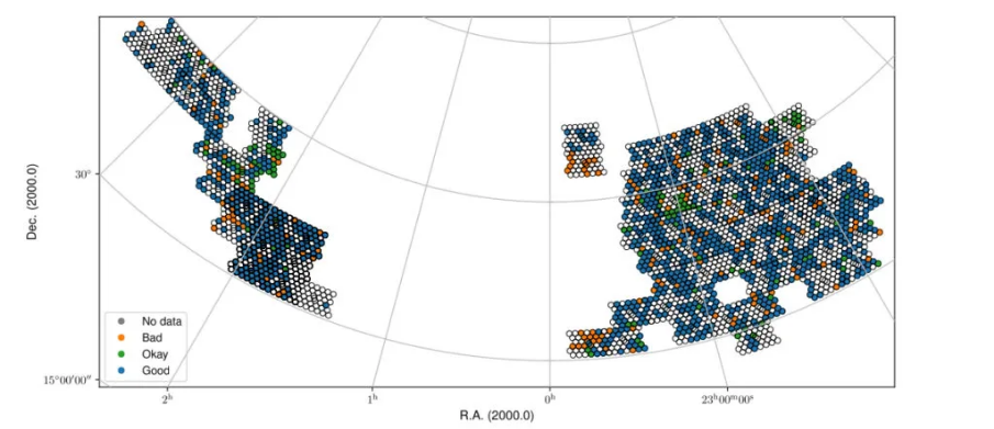
    Fig. 31 Fall sky view of the released data for cube0, color-coded by status (Good, Okay, Bad).

    Data Products

    Available data products

    Raw data Products

    Raw observational data

    The raw observational data is recorded in measurement-set (MS) format. A survey field observation consists of forty beams covering the field; with all dishes the size of this dataset is 4.6 TB. A set of calibration scans consists of 40 separate observations taken in succession. For each calibrator scan only one beam contains the calibrator. All other beams not containing the calibrator are discarded. These observations vary in between 3–5 minutes and the total datasize for a complete calibrator scan (all forty beams) is 64-106 GB. The calibrator observations are taken at a higher time resolution than the survey fields (10 vs. 30 seconds) to allow better RFI excision due to their shorter integration time. The raw data are stored in long-term storage at SurfSARA to enable future reprocessing with improvements to the Apercal pipeline.

    Inspection plots

    Upon ingest to ALTA, inspection plots showing various views of data quality are created. The majority of these plots show the behavior per compound beam, with different slices of the data to highlight different aspects of quality. Example inspection plots can be found here. These plots are:

    • Amplitude(all): Amplitude across all beams, averaged over all parameters
    • Amplitude f(time): Amplitude across all beams, concentric circles as a function of time inwards (start * to end)
    • Amplitude f(antenna): Amplitude across all beams, concentric circles as a function of antenna inwards (RT2 to RTD)
    • Amplitude f(baseline): Amplitude across all beams, concentric circles as a function of baseline inwards (in MS order)
    • Phase (all): Phase across all beams, averaged over all parameters
    • Phase f(time): Phase across all beams, concentric circles as a function of time inwards (start to end)
    • Phase f(antenna): Phase across all beams, concentric circles as a function of antenna inwards (RT2 to RTD)
    • Phase f(baseline): Phase across all beams, concentric circles as a function of baseline inwards (in MS order)
    • Amplitude vs time: Baseline plot of amplitude as function of time, coloured by MS order of baselines
    • Amplitude vs channel: Baseline plot of amplitude as function of channel, coloured by MS order of baselines
    • Phase vs time: Baseline plot of phase as function of time, coloured by MS order of baselines
    • Phase vs channel: Baseline plot of phase as function of channel, coloured by MS order of baselines
    • Waterfall: scaled amplitude : Waterfall plot of amplitude as a function of channel (x-axis) and time (y-axis),with fixed scaling
    • Waterfall: unscaled amplitude: Waterfall plot of amplitude as a function of channel (x-axis) and time (y-axis), no scaling
    • Waterfall: scaled phase: Waterfall plot of phase as a function of channel (x-axis) and time (y-axis), fixed scale
    • Waterfall: unscaled phase: Waterfall plot of phase as a function of channel (x-axis) and time (y-axis), no scaling

    In addition, there are plots for a single beam, either the central compound beam for a target observation or the compound beam containing a calibrator for calibrator observations showing a full view of the data. These plots are:

    • Beams XX: Waterfall plots of phase (upper right) and amplitude (lower left) for the XX polarization as a function of frequency (x-axis) and time (y-axis) for each baseline pair given by the antenna names (middle diagonal)
    • Beams YY: Waterfall plots of phase (upper right) and amplitude (lower left) for the YY polarization as a function of frequency (x-axis) and time (y-axis) for each baseline pair given by the antenna names (middle diagonal)

    Processed data products

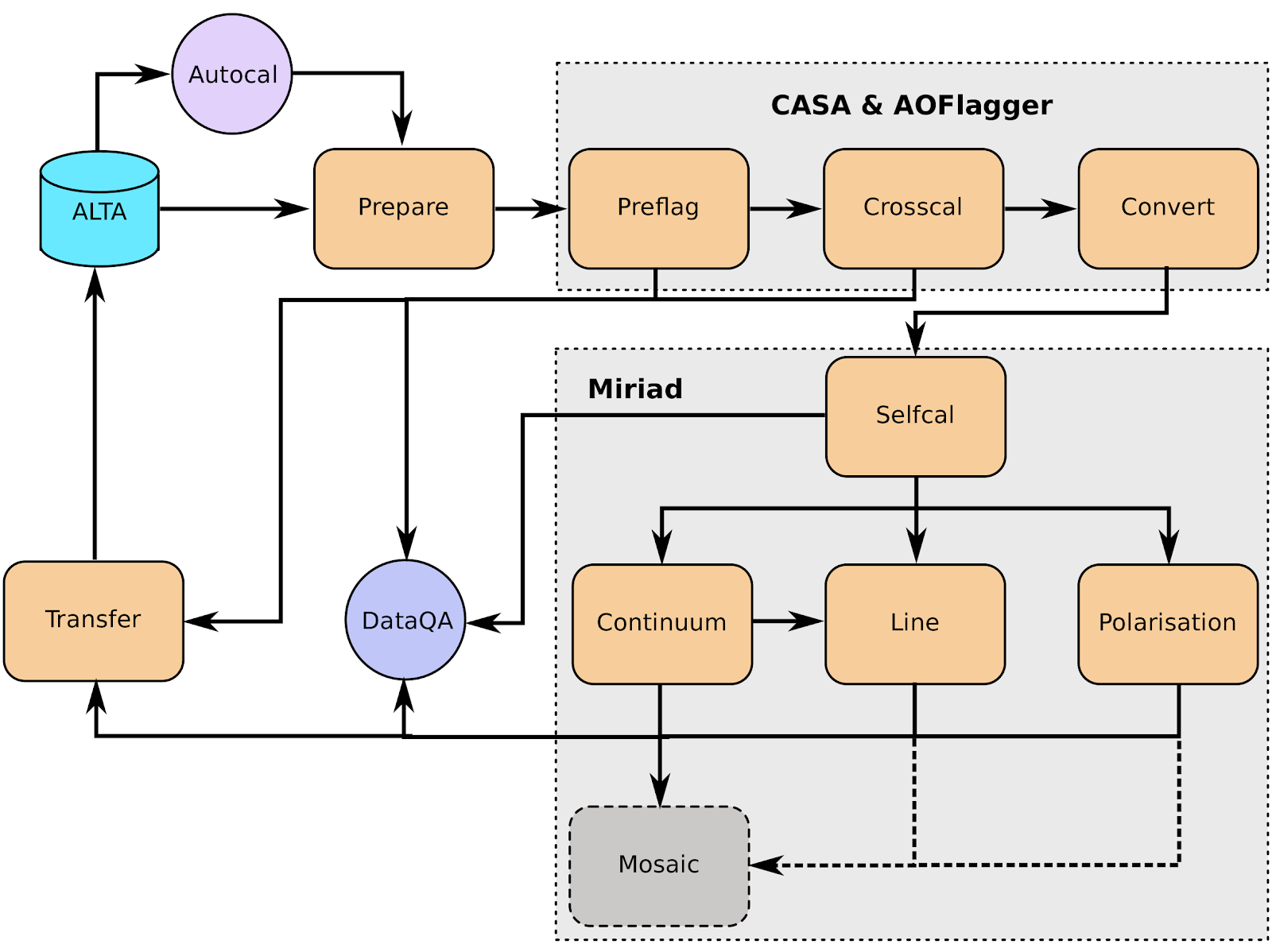
    The Apercal pipeline (see “Apercal overview and structure”) calibrates the data and produces final images and cubes per compound beam. All data products described below are for an individual compound beam, of which there are forty per observation. These data products are not primary-beam corrected; primary-beam images are provided separately (see the “Primary Beam Response” section, specifically “Released primary beam images”, and “User Interfaces”); these may be used for mosaicking or for correction of individual images.

    Processed data products are ingested back into ALTA on a per-beam basis, and in “Released processed data products” we motivate the choice to release data on a per-beam basis. Note that the release of a beam releases all processed data associated with that beam.

    An important note is that currently only the upper 150 MHz of the band is processed; thus the processed data products are produced over the range 1280-1430 MHz. Moreover, the first 12.5 MHz of data are flagged due to persistent RFI, therefore the resulting central frequency is 1361.25 MHz. The nominal bandwidth is then 137.5 MHz, but effectively it could be smaller due to additional RFI flagging. The (currently archived) data products are described below:

    • Calibration tablesThe crosscal module portion of Apercal produces calibration tables that can be applied to the original data to reproduce the cross calibration. These tables are in standard CASA/MS format and a summary of all the calibration tables is provided in Table 5 , where 3CFFF refers to a flux/bandpass calibrator (namely, 3C147 or 3C196; occasionally 3C295) and 3CPPP to a polarization calibrator (namely, 3C286 or 3C138).Calibration tables and naming scheme.
    • Global delays 3CFFF.K
      Bandpass solutions 3CFFF.Bscan
      Intermediary, initial phase solutions 3CFFF.G0ph
      Final complex gain solutions 3CFFF.G1ap
      Crosshand delay 3CPPP.Kcross
      Leakage terms 3CFFF.Df
      XY phase offset 3CPPP.Xf
    • Full time, Stokes and spectral-resolution calibrated visibility dataAfter the completion of the self-calibration, the final selfcal solutions are applied to the full spectral resolution uv data, and this uv dataset is written out as a UVFITS file as an intermediate data product. Currently, the final calibrated uv-data are stored at full time and spectral resolution for all polarizations; this may change with future updates to the processing pipeline.
    • Continuum imagesA multi-frequency Stokes I image is created over the full processed frequency range (currently 150 MHz; effectively less due to RFI occupancy) and saved as a FITS file for each beam. These images are 3.4°×3.4°(3073×3073 pixels, with 4′′/pixel). This samples well outside the primary beam response but is necessary to account for cases where a strong source is in a side-lobe and needs to be included in the self-calibration model and cleaning. Sources above 5-σ should be identified and cleaned to the 1-σ level.
    • Polarization images and cubes A multi-frequency Stokes V image over the full bandwidth is produced. This image matches the continuum image in spatial extent: 3.4°×3.4°(3073×3073 pixels, with 4′′/pixel). In order to prevent bandwidth depolarization and enable rotation measure synthesis studies, Stokes Q and U cubes with a frequency resolution of 6.25 MHz are produced. The cubes have a smaller spatial extent of 2.7°×2.7°(2049×2049 pixels, with 4′′/pixel).
    • Line and dirty beam cubes Four line cubes over a set of different frequency ranges are produced. Table 6 summarizes the covered frequency ranges and provides the corresponding redshift range for HI. The lowest redshift cube is produced at full spectral resolution while other cubes are produced with a 3-channel averaging. These cubes have a spatial extent of 1.1°×1.1°(661×661 pixels, with 6′′/pixel). As the Apercal pipeline does not provide source finding or cleaning of the line cubes, corresponding dirty beam cubes, with twice the spatial coverage, are also archived to allow offline cleaning of source emission. For cutting-down in archiving resources, taking advantage of the point symmetric structure, the dirty beam cubes have been reduced by a factor of two by cutting the beams in half. Informations how to recover to the full beam can be found here [https://github.com/apertif/trim_apertif_beam_cube]. Frequency/velocity coverage and resolution for all line cubes. Velocities use the optical definition and velocity resolutions are for the center frequency/velocity of each cube.
    • Cube0 1292.5 – 1337.1 18110 – 28226 0.062 – 0.099 36.6 8.3
      Cube1 1333.1 – 1377.7 9155 – 19005 0.031 – 0.065 36.6 8.1
      Cube2 1373.8 – 1418.4 424 – 10005 0.001 – 0.034 36.6 7.9
      Cube3 1414.5 – 1429.3 -1873 – 1250 0 – 0.004 12.2 2.6

    A summary of all the archived data products and their sizes (per beam and for a complete observation) are provided in Table 7 :

    Summary of archived data products, including their format and sizes. For visibility data, the dimensions are for polarization and frequency. For images and cubes, the dimensions are for spatial sizes and frequency (when appropriate). The calibrator visibility sizes are after pruning to keep only the Apertif beam that contains the calibrator, and the range of sizes reflects the different calibrator scan lengths.

    Survey field raw visibility data MS 4 x 24576 117 GB 4.7 TB
    Calibrator raw visibility data MS 4 x 24576 1.6-2.6 GB 64-104 GB
    Calibration tables MS table 660 MB 26.3GB
    Self-calibrated visibility data uvfits 4 x 12288 58 GB 2.3TB
    Multi-frequency synthesis beam images fits 3073 x 3073 37 MB 1.5 GB
    Stokes Q and U cubes fits 2049 x 2049 x 24 1.5 GB 62 GB
    Stokes V multi-frequency synthesis image fits 3073 x 3073 37 MB 1.5 GB
    Continuum-subtracted dirty line cubes fits 661 x 661 x 1218 8 320 GB
    Restoring beam cubes fits 1321 x 1321 x 1218 320 1.28 TB

    Validation of processed data products

    Continuum

    Image validation

    The continuum images were individually validated for every beam. In order to do this, a set of metrics was defined which inform on different aspects of image quality. The starting point of the validation are the residual images obtained after cleaning the continuum images. The validation aims at checking to what extent these images only contain Gaussian noise. The premise being that any significant deviation from this indicates issues with the calibration and/or the reduction of the data.

    The following parameters were derived for each residual image.

    • σ_in: Noise in inner half degree of the image, determined in a robust way from the residual image using the median of the absolute values.
    • σ_out Noise at the edge of the residual image, more than a degree from the centre determined in a robust way from the residual image using the median of the absolute values. This value is taken as a reasonable measure of the expected noise.
    • R=σ_in/σ_out: A measure of the strength of artifacts left in the centre of the residual image.
    • Ex-2: Area, in units of beam area, with values below 2 σ_out in the inner 0.5 degree of the residual image, in excess of what expected from a purely Gaussian distribution. For perfect noise Ex-2 = 0.
    • MaxNeg: the level, in units of σ_out, at which the area covered by pixels with values below this level is 10 beams. The expected value is -3.2. More negative values indicate significant negative calibration residuals.

    Note that we did not use the equivalents of the parameters Ex-2 and MaxNeg based on positive deviations from Gaussianity (Ex+2 and MaxPos). This is because many residual images have weak, positive residuals due to insufficient cleaning which would then dominate the validation.

    Visual examination of a large set of images was undertaken to define the numerical criteria that would catch significant image artifacts, as used above. The main types of image artifacts due to errors in the selfcalibration as well as strong direction-dependent errors for which the calibration pipeline did not attempt to correct. The criteria were set so that the large majority of images which were visually assessed as good would pass while only a small fraction of images that were visually assessed as bad would be classified as good.

    The final criteria used to reject images are: * R > 1.225. This criterion catches stripes due to errors in the amplitude calibration. * R > 1.15, MaxNeg < -4.5 and Ex-2>400. This criterion catches general image artifacts and deviations from Gaussianity in the residual image.

    Two additional criteria were set based on survey specifications: * σ_in or σ_out > 60 microJy/beam. In this case the noise of the image does not meet the minimum requirement to be considered survey quality and valid. * The minor axis of the restoring beam is > 15 arcsec. This occurs when both dishes RTC and RTD are missing from an observation. In this case, the required angular resolution of the survey is not met.

    Flux scale & astrometry

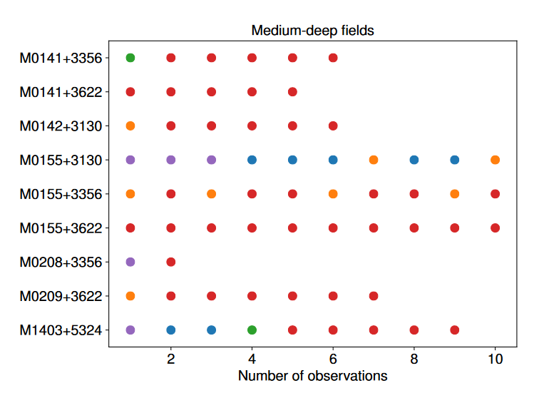
    For checking the consistency of the flux scale two beams of an observation of a field in the Perseus-Pisces region centered on RA(J2000) = 01h55m and Dec(J2000) = 33d56’ which was observed ten times between September 2019 and January 2020 were examined. The automatic source finder PyBDSF (also used in the Apercal pipeline) was used to find and determine source fluxes, positions and sizes and compared these from observation to observation. We restricted the comparison to sources that are less than 35” in size and have fluxes above 3 mJy (100 times the typical rms noise) and agree in position to within 3 arcsecs to ensure that the sources used for comparison are indeed identical and have been included in the clean masks.

    The overall consistency is very good with a mean of 1.014 and an rms of 4% . If one excludes the two most discrepant observations (ObsID 191207035 and 191227014) the rms decreases to 2%. Table 8 provides the flux ratio of 10 observations relative to the last observation made on 06.01.2020 (ObsID 200106010)

    The flux ratio of 10 observations relative to the last observation made on 06.01.2020 (ObsID 200106010)

    190919049 0.9982
    191207035 0.9311
    191223022 1.0041
    191225015 1.0116
    191227014 1.1069
    191229014 1.0185
    191231013 1.0062
    200102012 1.0446
    200104011 1.0222
    200106010 1.0000

    An example of two observations (ObsID 200106010 and 190909049, observed at 06.01.2020 and 09.09.2019 respectively) compared to one another is shown in Fig. 32. Plotted is the relative difference in flux versus the flux in the 06.01.2020 observation.

    Relative flux error
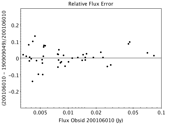
Fig. 32 Relative flux difference between the sources in a mosaic of ObsID 200106010 and a mosaic of ObsID 190909049 as a function of their flux measured in ObsID 200106010.

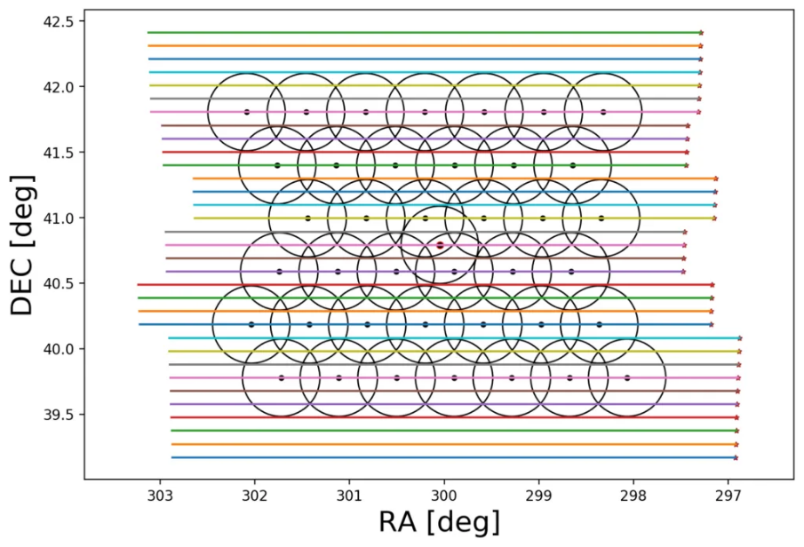
    To assess the agreement with the NVSS we made mosaics of the full field of view (40 beams) of all observations using the measured shapes of the 40 beams. The reason for using mosaics rather than individual beams was to have a large enough number of sources for the comparison as in an individual beam there usually are only of order a dozen that are bright enough. The mosaicing routine takes into account shapes of the beams made with the phased array feeds as determined from drift scans across Cygnus A (see the section on Primary beam response: Drift scan method) and corrects for the presence of correlated noise in adjacent beams. The mosaics were made with a resolution of 28” x 28”. We ran PyBDSF on the mosaics to produce a source catalog and compared sources in this catalogue with the sources in the NVSS source catalog extracted from VizieR. For the comparison we restricted ourselves to sources that agree in position to within 4”, are less than 28.5” in size and stronger than 3 mJy in the Apertif mosaic.

    Table 9 captures the comparison of the individual mosaics with the NVSS. For each ObsID the median flux ratio NVSS / Apertif is given. On average the Apertif flux scale is 3% above the NVSS flux scale for these mosaics with an rms of 4%. If the two most discrepant ObsIDs are omitted (191207035 and 191227014) the rms reduces to 2%. Fig. 33 illustrates the agreement between the Apertif and NVSS flux scale for ObsID 200102012. Since the observing frequency of the mosaic is 1360 MHz as opposed to the 1400 MHz of NVSS ~2% of the flux difference can be accounted for by spectral index effects (assuming an average spectral index of -0.7) which were not taken into account.

    Median flux ratio NVSS/Apertif for each ObsID

    190919049 0.943
    191207035 0.894
    191223022 0.962
    191225015 0.969
    191227014 1.083
    191229014 0.980
    191231013 0.974
    200102012 1.004
    200104011 0.976
    200106010 0.964

    A flux scale comparison using the beam shapes determined from a direct comparison of the DR1 observations with NVSS using a Gaussian process regression technique provides a better picture as all DR1 data are used rather than just one field.

    Relative flux error
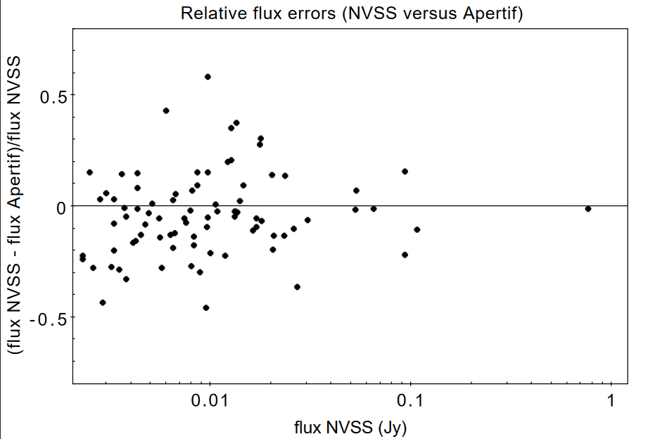
Fig. 33 Relative flux difference of sources in the NVSS catalogue and sources measured in an aperitif mosaic of ObsID 200102012 as a function of the flux of the sources in the NVSS catalogue

    This is described in “Characterization of the primary beams” and yields a current estimate of the flux scale of Apertif as compared to NVSS. From this comparison the Apertif fluxes are on average 9% higher than those of NVSS, accounting for a nominal spectral index of the sources of -0.7.

    Since we had to match sources in Apertif and NVSS for the source comparison we also obtained information on the agreement between the Apertif and NVSS astrometry. Fig. 34 shows the positional differences for sources in the mosaic of ObsID 200102012 and the NVSS catalogue. The agreement is very good with mean offsets of 0.05 +/- 0.2 arcsec in RA and -0.05 +/- 0.2 arcsec in Dec.

    Relative flux error

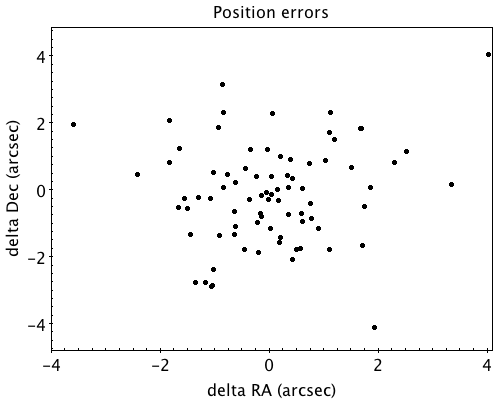
    Fig. 34 Position difference between the sources in the NVSS catalogue and the sources detected in the mosaic of ObsID 200102012.

    Polarization

    Validation of polarisation cubes/images

    Two types of polarisation products are generated by the pipeline. The first one being cubes of Stokes Q and U of 24 images each covering a bandwidth of 150 MHz resulting in a frequency resolution of 6.25 MHz. The second products are Stokes V images generated from the whole combined bandwidth of 150 MHz.

    Due to the different characteristics of these products two different sets of metrics were used to validate their quality. These metrics are very similar to the ones used for the continuum validation, but needed to be adjusted due to the following reasons:

    # Due to the physical nature of Stokes Q, U and V emission in the cubes can be a positive or negative quantity while it can only be positive in Stokes I. # Image artefacts are mostly influenced by the instrumental leakage characteristics of the primary beam in combination with direction dependent effects. This means that the strongest artefacts often appear for sources far away from the beam centres where the instrumental leakage is higher. # For Stokes Q and U even faint artefacts in individual images can stack up if those are present over the whole cube at a similar position once the RM-Synthesis technique is applied in later stages of the analysis. This is also possible vice versa where strong artefacts in an individual image can be averaged out in this process and lead to a good image quality after RM-Synthesis processing. # Stokes V represents the circular polarisation. Astronomically circularly polarised sources are extremely rare and most often show percentage polarisation of below 1%, so that Stokes V images should normally be regarded as empty.

    In the following we describe the sets of metrics and the determined values for the quality assurance of the polarisation cubes/images. All values and the validation information for released beams is available in the table of the survey data release for polarisation observations.

    Stokes V validation

    The following parameters were derived for each Stokes V image:

    • σ_in: rms in the inner part of the image, which is defined as a radius of <30′ around the central coordinate of a beam [microJy/beam]
    • σ_out: rms in the outer part of the image, which is defined as a radius of >60′ around the central coordinate of a beam [microJy/beam]
    • FT_max: Absolute of the Fourier Transformation of the image. This value gives a good measure of repeating structures in the image such as amplitude artefacts which manifest as stripes.
    • peak_inner: The maximum of the absolute values of the inner part of the image as defined in σin (see above) [microJy/beam]
    • b_min: The diameter of the FWHM minor axis of the synthesised beam [arcseconds]

    A Stokes V image fails validation if one of the following criteria is met:

    # σ_in and/or σ_out > 60 microJy/beam. This is the same value as for the continuum validation. # b_min > 15’’. This criterium filters any images for observations where failing or missing dishes are raising the FWHM of the synthesised beam above a value which is not acceptable for the survey. # FT_max > 25. This value was empirically determined and filters any image, which is suffering from leftover RFI or strong amplitude errors. # peak_inner > 4mJy. Images with values above this limit are most likely strongly affected by instrumental leakage and in most cases also show strong artefacts.

    The first two criteria match that of the continuum validation and are based on survey specification. The second two criteria were empirically determined to filter images with strong polarization artefacts. Stokes Q&U validation

    Stokes Q/U cubes are validated depending on how many planes in a cube fail the following two criteria:

    # The synthesised beam’s minor axis of an image is larger than 17.5’’. We are using a slightly larger value here compared to the continuum or Stokes V validation due to the fact that the beam becomes larger for images at lower frequencies. # The rms noise in an image is larger than 300 microJy/beam. This corresponds to the same noise level as for the continuum and Stokes V images assuming a homogeneous noise distribution along the frequency axis. Stacking 24 images would reduce the noise by a factor of ~5.

    Beams where more than one third of the images (>8) in Stokes Q or U are failing either of the above mentioned criterium do not pass the validation.

    The table of released polarisation beams includes the following columns that describe the Stokes Q/U data quality:

    • Qbeam_frac: Fraction of Q image planes failing criterium 1. [0.0-1.0]
    • Ubeam_frac: Fraction of U image planes failing criterium 1. [0.0-1.0]
    • Qnoise_frac: Fraction of Q image planes failing criterium 2. [0.0-1.0]
    • Unoise_frac: Fraction of U image planes failing criterium 2. [0.0-1.0]

    HI

    Cube Validation

    The quality of the HI line data was validated in multiple steps. We concentrate the analysis on cubes 0, 1, and 2 (see Table 6 in the “Available data products” document for the frequency ranges of the cubes), as the quality of cube 3 always followed that of cube 2 due to both of them being in adjacent low-RFI frequency ranges.

    As a first step all cubes 0, 1, and 2 where the average rms noise was larger than 3 mJy/beam were rejected. Inspection of the cubes showed that such large noise values always indicates the presence of major artefacts in the cube.

    We then constructed noise histograms for cubes 0, 1 and 2 of each observation and beam combination. We made no attempt to flag any sources prior to determining the noise histogram. The HI cubes are mostly empty (i.e. consist of noise pixels) and real sources have no discernible effect on the histogram. The only exception is that all cubes 0 were blanked below 1310 MHz to remove the impact of residual RFI at these frequencies.

    We also extracted representative channels as well as position-velocity slices from each cube. The cubes of 14 observations (~550 cubes) were inspected by eye for the presence of artefacts and to gauge the impact and effect of data artefacts on the noise histograms.

    Artefacts generally fell in two categories: due to imperfect continuum subtraction and due to imperfect sub-bands, which we discuss in turn.

    • Continuum subtraction artefacts

    Continuum subtraction artefacts (and with it the presence of residual grating rings) add broad wings with extreme positive and negative values to the noise histogram. Trial and error showed that these wings could be robustly detected by quantifying the fraction fex of the total number of pixels with an absolute value flux value >6.75σ where σ is the standard rms noise in the cube. While adding wings of extreme value pixels to the histogram, these artefacts in general do not affect the Gaussian shape of the central part of the histogram (i.e., at low σ values).

    • Sub-band artefacts

    The presence of sub-bands with lower quality (i.e., a higher noise) manifests itself not by wings of extreme pixels but by a systematic change in the shape of the histogram through the addition of “shoulders” to the histogram (lower kurtosis). Trial and error showed that the presence of these features were best detected by comparing the rms width of the histogram with that at the level of 0.8 percent of the maximum of the histogram. We define the parameter p0.8 or the ratio of this 0.8 percent width and the rms.

    We compared our “good”, “bad” or “OK” rankings as determined by eye for the 14 observations with the corresponding fex and p0.8 values. This is illustrated in Fig. 35 where we show the distribution of all cubes 2 in the fex-p0.8 plane with the cubes which we inspected by eye color coded to indicate their quality ranking.

    “Good” cubes, i.e., those with no or very minor artefacts, were concentrated in a small part of parameter space obeying the following criteria:

    • rms < 3 mJy/beam
    • log(fex) < -5.30
    • p0.8 < 0.25 fex + 5.875

    A second criterion defines cubes of OK quality, containing some minor artefacts. This consists of cubes meeting the following conditions:

    • rms < 3 mJy/beam
    • -5.30 < log(fex) < -4.52
    • p0.8 < 0.5 fex + 7.2

    The upper limit of -4.52 of the second condition is not a hard limit and a slightly different value could also have been chosen. We found however that the values used here give a good compromise in minimizing the number of false qualifications of “OK” cubes

    Cubes not obeying any of these two sets of criteria were considered “bad”. Using these conditions we defined for all cubes 0, 1 and 2 a subset of good and OK cubes. Cube 3 in all cases follows the quality designation of cube 2.

    Fig. 36 shows the noise histograms and a representative channel map and position velocity slice for each of the three quality categories.

    Whether a cube is part of the data release is determined by the quality criteria of the corresponding continuum image. This is described in more detail in the document “Released processed data products”. The quality of each cube and the metrics used to determine that quality are included in the VO table describing the released HI observations (see “User Interfaces”).

    Relative flux error
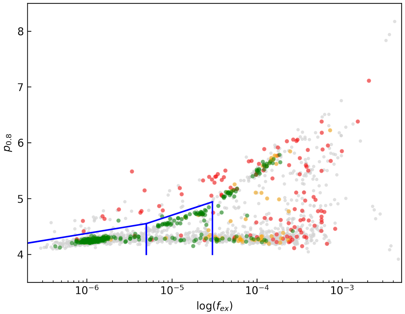
Fig. 35 Distribution of cubes 2 of all beams in the fex-p0.8 plane (grey points). Overplotted are quality assessments of the beams of 14 observations. Good cubes are indicated by green points, OK by orange points and bad cubes by red points. The blue lines indicate the regions where cubes are considered good (left region) or OK (right region).

    Relative flux errorFig. 36 Examples of the three quality classes used for the HI quality assessment. The top row shows an example of a “good” observation (Obsid 200202012, beam 17, cube 2), the middle one an “OK” observation (Obsid 200202012, beam 33, cube 2) and the bottom one a “bad” observation (Obsid 200202012, beam 20, cube 2). The columns show, from left to right, the noise histogram, an extract of the central velocity channel, and a position-velocity diagram through the center of the cube. In the plots in the left column the short horizontal line at the top indicates the rms. The two dotted vertical lines indicate the ±6.75 x rms values. The “good” observation in the top row shows hardly any artefacts and a Gaussian noise histogram. The “OK” observation in the middle row shows a minor continuum subtraction artefact (which in turn causes somewhat extended wings to the noise histogram). The “bad” observation in the bottom row shows major continuum subtraction artefacts, resulting in a very non-Gaussian histogram.

    External comparison

    In order to further validate the line cubes, we performed preliminary source finding and cleaning of a subset of cubes using SoFiA-2 (Source Finding Application; Serra et al. 2015, https://github.com/SoFiA-Admin/SoFiA-2). Full details of this procedure are supplied in Hess et al. (in prep).

    Comparison to ALFALFA

    We compared the properties of HI detections in Apertif with the properties of HI detections in the ALFALFA catalogue (Haynes et al. 2018). We created a source catalogue with SoFiA and cross matched the detected sources with the ALFALFA catalogue. In 21 fields that overlap in the footprint of both surveys, we found 479 matching sources. Out of these, 336 sources were found in data cubes with “good” quality, 39 in data cubes with “OK” quality and 104 were found in “bad” quality data cubes. The results of the comparison are shown in Fig. 37 and Fig. 38. The color coding of these figures reflects the quality of the data cube in which the sources were identified with blue for “good”, green for “OK” and orange for “bad”.

    Overall the properties of the Apertif detections agree well with the ALFALFA detections. There are some sources that have smaller line widths (w20) than the ALFALFA sources. This is likely connected to the flagging of 3 channels out of every 64 because of the strong dropoff in response (See “Aliasing” in “System notes”). Cubes 0, 1, and 2 have every three channels averaged together. Combined with the flagging of three channels out of every 64, this means that every 22nd channel in these cubes has no signal, and there are channels with ⅓ nominal sensitivity (periodicity of 42 and 21 channels) and ⅔ nominal sensitivity (periodicity of 63 channels). These flagged or partially flagged channels can result in a source being spectrally separated into two different detections. This then also results in smaller line widths for these sources. Another reason for the smaller line widths in Apertif can be extended emission detected in ALFALFA that gets filtered out by the interferometry.

    Relative flux error
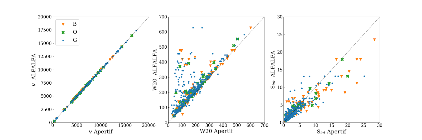
Fig. 37 Comparing the properties of overlapping Apertif and ALFALFA sources. First panel: systemic velocity, second panel: W20 line width, third panel: integrated flux. The different colored markers represent sources detected in “good” (G), “OK” (O), and “bad” (B) quality HI data cubes.

    Relative flux error
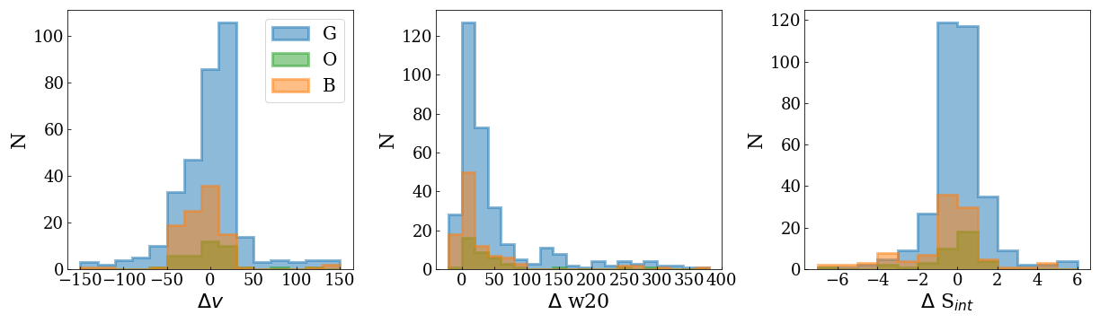
Fig. 38 Distribution of the difference in systemic velocity, W20 and integrated flux between Apertif and ALFALFA detections. The colors represent detections in “good” (G), “OK” (O), and “bad” (B) quality HI data cubes.

    User Interfaces

    The Apertif Data Release 1 (Apertif DR1) is hosted on the Apertif Long Term Archive and exposed to the community through the standard Virtual Observatory protocol. This section describes how the Apertif DR1 data products can be queried and accessed by using different applications.

    Introduction

    The science-ready data products as described in Available data products and Released processed data products are exposed through standard Virtual Observatory protocols to facilitate their access and exploration.

    The Apertif DR1 data is hosted on the Apertif Long Term Archive (ALTA) system. We recommend astronomers to use the VO interfaces described below for data discovery. These interfaces will redirect to ALTA file servers for data access where appropriate.

    In particular, the protocols offered are the Tabular Access Protocol (TAP), Simple Application Messaging Protocol (SAMP) and the Simple Image Access protocol (SIA). TAP and SAMP enables queries to explore the data in a tabular form using tools such as TOPCAT. TOPCAT is an interactive graphical viewer and editor for tabular data, it enables the interactive exploration of large tables performing several types of plotting, statistics, editing and visualization of tables. SIA enables the rapid display of images and cubes through all sky atlas tools such as ALADIN. ALADIN is an interactive sky atlas allowing the user to visualize digitized astronomical images/cubes and superimpose entries from astronomical catalogues or databases.

    The data published in the VO can also be accessed using a web browser at https://vo.astron.nl. This web interface provides a page on which all the collections present in the registry are listed, including the published Apertif DR1 data sets (Fig. 39).

    Relative flux errorFig. 39 ASTRON VO interface.

    Selecting a data collection allows the user to perform a cone search through a webform (Fig. 40) for all data products of that given class overlapping a given pointing. The size of the continuum images as well as the cubes extend beyond the 10% primary beam level for cleaning the secondary lobes of bright offset sources. To ensure that the search is done in the area of maximum sensitivity the search is performed on a maxim radius of 0.75 degrees from the center (this represents the average value of where the sensitivity drops). This value can be modified using the Max distance from center. A different output with respect to the default can be customized using More output fields selection button.

    Relative flux error

    Fig. 40 Query search form for continuum images.

    The result is a table in the requested output format in which every row corresponds to a data product (Fig. 41).

    In each row there is a column, Product key, which is a link that allows the user to download the fits file of the image or the cube of interest.

    The selected target and the position of the individual beams can be visualized using the Quick plot button at the top of the window of the results of the search query (Fig. 41).

    In the column Related products another link connects to a page containing a list of links to additional related data that can be useful to interpret or reanalyze that given product (e.g. primary beam images), for which a preview is provided (Fig. 42).

    Relative flux error

    Fig. 41 Result of the search query.

    Relative flux error

    Fig. 42 Links of ancillary data products related to the target of interest.

    The columns shown in Figure 3 are the most informative for the astronomers (e.g. position, observing frequency, observing date, quality assessment, format etc), please note that more columns are available but not displayed here. The complete set of columns can be visualized via topcat as described below or using More output fields selection button in the search query. Querying the released data is also possible using e.g. TOPCAT using TAP. Via the TAP protocol, it is possible to query the registry in a more flexible way using an enriched SQL syntax called ADQL. An example is given in Fig. 43 : click the link indicated with the red ellipse on the left panel Try ADQL and place your ADQL query on the query form.

    Relative flux error

    Fig. 43 ADQL query form.

    The table names to use in the query form of Fig. 43, are summarized in Table 10. The URL for the query is then: https://vo.astron.nl/apertif_dr1/q/{Table name}/form (e.g. http://vo.astro.nl/apertif_dr1/q/apertif_dr1_continuum_images/form}.

    It is possible to query all the available dataproducts at once by using the table ivoa.obscore and by appending to the ADQL statement “where obs_collection=” it is possible to limit the search to the apertif_dr1 only.

    VO-Apertif DR1 Processed Data Products

    Table names to be used in the ADQL query.

    Table name obscore type obscore subtype
    apertif_dr1.continuum_images image continuum
    apertif_dr1.pol_cubes cube polarization cube
    apertif_dr1.spectral_cubes cube spectral cube
    apertif_dr1.beam_cubes cube dirty beam

    Access via TOPCAT

    The Apertif DR1 data collection tables can be accessed using TOPCAT, an interactive graphical viewer and editor for tabular data. The data can be sent from vo.astron.nl to TOPCAT using one of the two protocols: SAMP or TAP. The two subsections below provide a description on how to access the tabular data using either SAMP(link to Send via SAMP subsection) or TAP(link to VO Table Access Protocol (TAP) subsection).

    Send via SAMP

    With TOPCAT opened, and once you are satisfied with the output of the cone search in the Astron VO webform, click the grey button “Send via SAMP” as shown on the top of the output list of Figure 3. Authorize the connection and wait until the download is completed.

    Once completed, the catalogue will be visible in the left panel of TOPCAT (Table List). Click on the new entry as shown by the arrow in Fig. 44. At this point the table browser will open showing the content of the DACHS results (PLACE HOLDER use DR1 in selection). From here any TOPCAT tool can be used for further inspection and analysis of the results. Alternatively the table can be saved in various formats and used locally with other programs (e.g. python scripts etc).

    Relative flux error

    Fig. 44 TOPCAT table browser view of the Apertif DR1 data collection tables.

    VO Table Acess Protocol (TAP)

    From the TOPCAT menu bar, select VO and in the drop down, select Table Access Protocol (TAP) as shown by the red arrow in Fig. 45.

    This will open the Table Access Query window where the ASTRON VO TAP server is listed. Select it and click on Use Service at the bottom of the window (Fig. 46). Another tab will open showing the Apertif DR1 data collection. Select one, e.g. continuum image, and enter a query command in the bottom panel, an example of which is indicated by the red arrow in Fig. 47. Submit the query using Run Query. This will show the resulting table in the Table list view shown before in Fig. 44. From here, any TOPCAT tool can again be used. As mentioned in the previous section, the query result in vo.astron.nl will display a subset of the columns of the Apertif DR1 table (e.g. position, observing frequency, observing date, quality assessment, format etc). The complete set of columns (e.g. pipeline version, wcs references etc) belonging to each data collection of the Apertif DR1 can be explored using the option described in this section.

    The position of the targets can be visualized using the option skyplot in TOPCAT, once the search query has been sent via SAMP or TAP as described in this section.

    Relative flux error

    Fig. 45 TOPCAT menu bar for VO services.

    Relative flux error

    Fig. 46 TOPCAT TAP service query form.

    Relative flux error

    Fig. 47 TOPCAT menu bar for VO services. Click for a bigger image.

    Another useful way to inspect the Apertif DR1 data collection, but also other data collections exposed via the ASTRON-VO, is the ivoa-obscore table. The same selection as before can be used (Fig. 47) but instead of selecting Apertif_dr1 tables, the table ivoa.obscore is to be selected. In this way it is possible to glance over all the data collections exposed via the ASTRON-VO. This might be useful for instance to enable multi-wavelength science exploring LOTSS and Apertif DR1 data or, as mentioned in the case of the ADQL query, to visualize multiple data collections at once.

    Having ALADIN open, and once you are satisfied with the resulting table, it can be sent to ALADIN following the instructions of Fig. 48.

    Relative flux error

    Fig. 48 How to transfer the TOPCAT query results to ALADIN.

    Access via ALADIN

    Catalogues

    The Apertif DR1 VO data collection can also be discovered directly via ALADIN either via simple image access protocol (SIAP) or tabular access protocol (TAP). The examples shown here require the desktop version of ALADIN.

    Open ALADIN and on the left panel for SIAP: select Others > SIA2 > astron.nl > The VO @ASTRON SIAP Version 2. Alternatively for TAP select Others > TAP > astron.nl > The VO @ASTRON TAP service (Fig. 49). A pop-up window will open. Click load, and enter a query using the Server selector (Fig. 50) or TAP access with astron.nl/tap (Fig. 51) to select the target of interest for SIAP and TAP respectively.

    Relative flux error

    Fig. 49 ALADIN display panel.

    Relative flux error

    Fig. 50 ALADIN server selector panel for SIAP.

    Relative flux error

    Fig. 51 ALADIN TAP access panel.

    After loading, the data collection catalogues can be plotted on the main panel by selecting them first on the right panel (e.g. highlighted in blue in Figures 14 and 15) and then by selecting the regions of interest on the bottom panel as shown in Figures 14 and 15. From here the usual functionality of ALADIN can be used.

    Relative flux error

    Fig. 52 Example of data collection selection via SIAP in ALADIN.

    Relative flux error

    Fig. 53 Example of data collection selection via TAP in ALADIN.

    Images

    Downloading images or cubes in ALADIN is also possible (see Fig. 54). The user will need to click on the url-link in the column access_url of the bottom panel. Then, once the image is loaded, click on the right panel as shown in Fig. 54. From here the usual functionality of ALADIN can be used.

    Relative flux error

    Fig. 54 Example of image selected from the Apertif DR1 displayed in ALADIN.

    Access to raw and calibrated visibilities

    Raw observations and calibrated visibilities can be discovered in the data collection as shown in Fig. 39, using the ASTRON-VO query form (Fig. 40) or via TAP using TOPCAT.

    In addition, the query results via ASTRON VO for continuum images, polarization images/cubes, and HI spectral cubes provides a link to ancillary data (Fig. 42), including raw and calibrated visibilities.

    These data products are stored on tape and not directly accessible for download, but until further notice access can be requested via the helpdesk (Fig. 56). The request will be processed on a best effort basis. Within the same request also the calibration tables can be made available (see “Available data products”).

    Relative flux error

    Fig. 55 Visibility data access page.

    Relative flux error

    Fig. 56 Astron help center webpage.

    Primary beam images

    The continuum images, HI spectral cubes and V images and Q&U cubes are not primary beam corrected. Primary-beam images may be used for mosaicking or for correction of individual images. More information about the primary beam images for Apertif, including their derivation, can be found in the “Overview of primary beam shapes for Apertif”. Specifically, “Released primary beam images” describes the primary beam images initially made available as part of this data release. As for other ancillary data products, primary beam images can be found in the query results following the links in the column Related products (Fig. 57) for continuum images, HI spectral cubes or polarization cubes.

    Relative flux error

    Fig. 57 Links to ancillary data.

    Python access

    The data collection and the table content can be accessed directly via python using the pyvo tool. Working directly in python the tables and the data products can be simply queried and outputs can be customized according to the user’s needs, without the involvement of TOPCAT or ALADIN.

    An example of a TAP query and image download can be found in the python script below (it has been tested for python 3.7). The result of the query can also be plotted using python.

    #To start you have to import the library pyvo (it is also possible to use astroquery if you want)
    import pyvo
    
    ## To perform a TAP query you have to connect to the service first
    tap_service = pyvo.dal.TAPService('https://vo.astron.nl/__system__/tap/run/tap')
    
    # This works also for
    form pyvo.registry.regtap import ivoid2service
    vo_tap_service = ivoid2service('ivo://astron.nl/tap')[0]
    
    # The TAPService object provides some introspection that allow you to check the various tables and their
    # description for example to print the available tables you can execute
    print('Tables present on http://vo.astron.nl')
    for table in tap_service.tables:
     print(table.name)
    print('-' * 10 + '\n' * 3)
    
    # or get the column names
    print('Available columns in apertif_dr1.continuum_images')
    print(tap_service.tables['apertif_dr1.continuum_images'].columns)
    print('-' * 10 + '\n' * 3)
    
    ## You can obviously perform tap queries accross the whole tap service as an example a cone search
    print('Performing TAP query')
    result = tap_service.search(
     "SELECT TOP 5 target, beam_number, accref, centeralpha, centerdelta, obsid, DISTANCE(" \
         "POINT('ICRS', centeralpha, centerdelta),"\
         "POINT('ICRS', 208.36, 52.36)) AS dist"\
     " FROM apertif_dr1.continuum_images"  \
     " WHERE 1=CONTAINS("
     "    POINT('ICRS', centeralpha, centerdelta),"\
     "    CIRCLE('ICRS', 208.36, 52.36, 0.08333333)) "\
     " ORDER BY dist ASC"
     )
    print(result)
    
    # The result can also be obtained as an astropy table
    astropy_table = result.to_table()
    print('-' * 10 + '\n' * 3)
    
    ## You can also download and plot the image
    import astropy.io.fits as fits
    from astropy.wcs import WCS
    import matplotlib.pyplot as plt
    import requests, os
    import numpy as np
    
    # DOWNLOAD only the first result
    #
    print('Downloading only the first result')
    file_name = '{}_{}_{}.fits'.format(
     result[0]['obsid'].decode(),
     result[0]['target'].decode(),
     result[0]['beam_number'])
    path = os.path.join(os.getcwd(), file_name)
    http_result = requests.get(result[0]['accref'].decode())
    print('Downloading file in', path)
    with open(file_name, 'wb') as fout:
     for content in http_result.iter_content():
         fout.write(content)
    hdu = fits.open(file_name)[0]
    wcs = WCS(hdu.header)
    # dropping unnecessary axes
    wcs = wcs.dropaxis(2).dropaxis(2)
    plt.subplot(projection=wcs)
    plt.imshow(hdu.data[0, 0, :, :], vmax=0.0005)
    plt.xlabel('RA')
    plt.ylabel('DEC')
    plt.show()

    Export machine readable table

    There are multiple ways to export a catalog of the various data products of the data release. On the vo.astron.nl pages, the results of a query can be exported to a csv file or fits table; running an empty query with a table limit of 5000 or more will return all entries.

    TOPCAT and the pyvo interface demonstrated above also provide functionality for exporting machine-readable files.

    The ADQL form is another option, and below we provide an example query that also provides information about the calibrators used for each beam. This query is specific to the continuum_images data product but can be adapted to other (beam-based, processed) data products by replacing the table name, e.g., for polarization cubes/images use pol_cubes (see Table 10 for a full list of the available tables).

    select data.*,
    flux_cal.obsid as flux_calibrator_obs_id,
    pol_cal.obsid as pol_calibrator_obs_id  from apertif_dr1.continuum_images data
    join  apertif_dr1.flux_cal_visibilities flux_cal on data.obsid=flux_cal.used_for and data.beam_number=flux_cal.beam
    join apertif_dr1.pol_cal_visibilities pol_cal on data.obsid=pol_cal.used_for and data.beam_number=pol_cal.beam
    order by obsid

    Data Usage Policy

    Papers making use of this data should include the following acknowledgement:

    This work makes use of data from the Apertif system installed at the Westerbork Synthesis Radio Telescope owned by ASTRON. ASTRON, the Netherlands Institute for Radio Astronomy, is an institute of the Dutch Research Council (“De Nederlandse Organisatie voor Wetenschappelijk Onderzoek, NWO).

    In addition, they should include the Apertif DR1 PID:

    http://hdl.handle.net/21.12136/B014022C-978B-40F6-96C6-1A3B1F4A3DB0

    and cite the imaging survey data release paper. This is not yet available but should be soon. Until then, it can be referenced as:

    Adams, E. A. K., et al. “First release of Apertif imaging survey data”, in prep.

    @astron

    SDC Helpdesk